Deep learning
Contents
22. Deep learning
While we promised that this chapter would not be a catalog of different machine learning methods, no book introducing machine learning – and particularly applied to a topic so closely bound with image processing – would be complete without at least a brief mention of deep learning. Deep learning is a relatively new branch of machine learning that encompasses a set of techniques that combine advances in artificial neural networks with clever optimization methods and large amounts of data to do remarkably well at many different machine learning tasks. We’d hesitate to call these methods “artificial intelligence” (AI), but these algorithms are prone to doing things that until recently we would have thought only humans can do, like recognize objects in a photograph, generate (at least somewhat) cogently written prose, or play Go. So we think that it’s fair to say that it’s the closest we’ve gotten to AI so far.
22.1. Artificial neural networks
It is only too appropriate that we would use a model of a neural network to study the brain. A deep learning algorithm is composed of individual functional units that are connected to each other to simulate a kind of simplified neural network. Just like real neurons, each unit in the network receives inputs – either from outside the network, or from other units in the network, and has outputs – into other neurons or as the final output of the network. Let’s look at a diagram of a very simple artificial neural network:
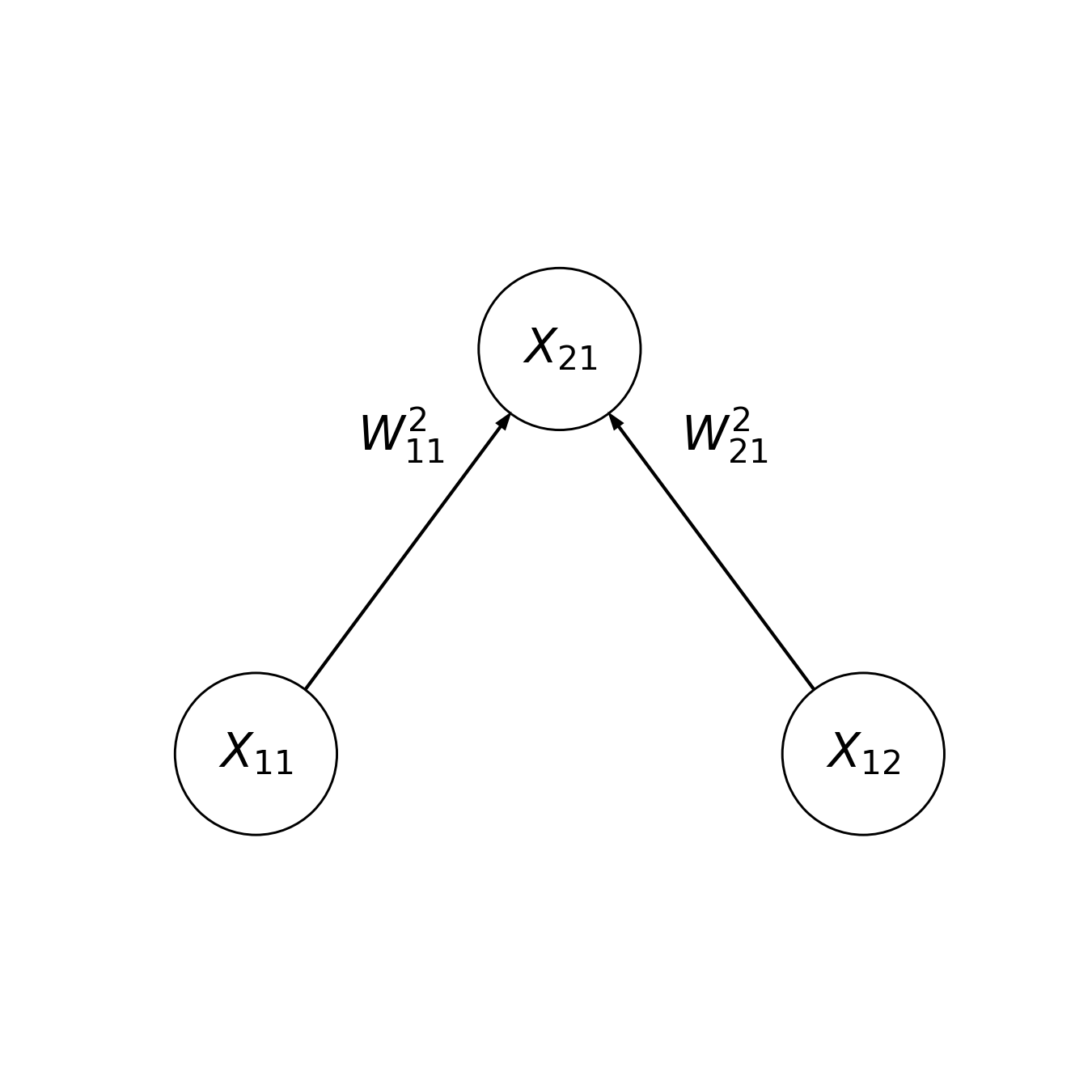
The circles denote nodes and the lines denote direct connections between nodes. The activity of the nodes at the bottom (denoted by \(X_{11}\) and \(X_{12}\)) is set by two different inputs to the network, and the activity of the node at the top (denoted by \(X_{21}\)) is the output of the network. The input layer is similar to the \(X\) matrix that you saw in previous chapters, with different rows of the matrix corresponding to different instances of the input. In this network, \(X_{21}\) is akin to the model predictions in the previous chapters. As an example, \(X_{11}\) might be the weight of an animal, \(X_{21}\) might be the wingspan of the animal, and \(X_{21}\) might be the model output: the predicted airspeed of the animal. This is the familiar regression setting that you saw in previous chapters with two inputs and one output.
In the notation we will use here, the first subscript indicates the layer number and the second subscript indicates the number of the particular unit within the layer. So, \(X_{12}\) is the second unit in the first layer, and \(X_{21}\) is the first unit in the second layer.
The activity in each unit in the input layer affects the activity in the output unit through a weight: \(W^2_{11}\) and \(W^2_{12}\). The notation for the weights is that the superscript tells us which layer these weights go into, the first subscript tells us the identity of the source unit and the second subscript tells us the identity of the target unit. For example, \(W^2_{11}\) is a weight from unit 1 in the first layer to unit 1 in the second layer and \(W^2_{21}\) is the weight from unit 2 of the first layer to unit 1 of the second layer.
How do the weights affect the activity in the second layer? In the simplest case: \(X_{21} = W^2_{11} X_{11} + W^2_{21} X_{12}\). That is, the activity in the second layer is the weighted linear sum of the activities in the first layer, where the activity in each unit is multiplied by the weight between that unit and the output.
22.1.1. Implementing a neural network
Written out in code, this might look something like the following. We use a
notation very similar to the one we used in writing out the math, where, for
example, \(X_{11}\) is written as x_11 and \(W^{2}_{11}\) is written as w_2_11.
x11 = 100
x12 = 40
w_2_11 = -1
w_2_21 = 3
x21 = w_2_11 * x11 + w_2_21 * x12
print(x21)
20
In our previous example, this might mean that the airspeed of an animal that weighs 100 grams and has a wingspan of 40 cm, might fly at a speed of 20 km/h (try out different numbers to see how speed is affected by these two factors, given these weights).
Neural networks become more sophisticated when we add more layers to them. For example, here is a three-layer network. There are two units in the input layer, two units in the hidden layer, and one unit in the output layer.
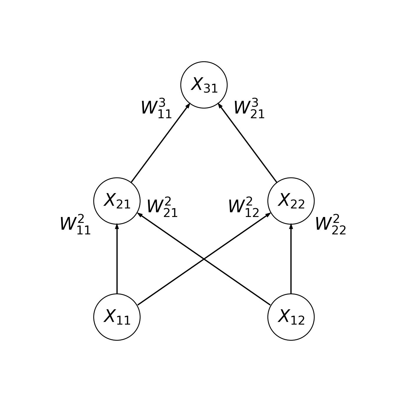
22.1.1.1. Exercise
Implement the code that calculates the output of this network, using the same notation that we used before. Don’t worry about the values of the weights – just make something up.
22.1.2. Activation functions
Another thing that adds power to neural networks is the addition of non-linear activation functions to the units. Schematically, it would look like this:
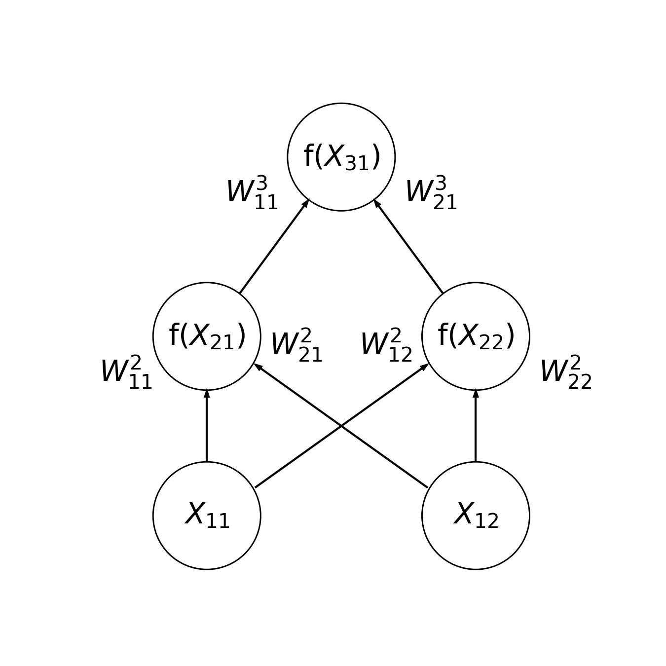
Where \(f()\) is the activation function. In each unit, this is applied to the weighted sum of the inputs. Often, a non-linear activation function is used to give the units a threshold of activity that would stimulate them to a response – just like a biological neuron! For example, one typical function to use would be a hyperbolic tangent, which changes very little for very small or very large values, and changes gradually in between. In this case, the output of the first unit in the hidden layer is \(tanh(W^2{11} X_{11} + W^2{12})\). Another non-linear activation function, that is often used in practice, is the rectified linear unit, or ReLU. This function sets the activations that are negative to zero and passes through activations that are positive as they were. We can write this function in Python in very few lines of code
def relu(x):
    if x < 0:
        return 0
    else:
        return x
And incorporate this into our two-layer network. In this case, adding the ReLU did not change the output of the network. This is because the output was positive. But you can try changing the weights to see what happens when the weighted sum \(W^2{11} X_{11} + W^2{12}\) becomes negative.
x11 = 100
x12 = 40
w_2_11 = -1
w_2_21 = 3
x21 = relu(w_2_11 * x11 + w_2_21 * x12)
print(x21)
20
22.1.2.1. Exercise
Add the ReLU function as an activation to the hidden and the output layer of the three-layer network that you previously implemented.
22.2. Learning through gradient descent and back-propagation
How do we know what values to assign to the weights of a neural network so that the input-output relationships are accurate? This is the goal of learning with these algorithms. This is implemented using two main ideas. The first idea is that of gradient descent. This mechanism for learning is similar to the optimization procedures that we used to fit machine learning models earlier in this chapter, or that we used to register images to each other in Section 16. It usually starts with some (often random!) guess of what the values of the weights should be and then – based on observations of training data – it determines a small change that should be introduced to improve the accuracy of the input-output relationship: the difference between the true value of \(y\) for each training sample, and the predicted value of \(y\), given the current values of the weights. In each round of training, the weights are adjusted gradually, based on the gradient of the weights with respect to the error. The gradient refers to the overall set of changes to the weights that improve the error and we descend in the direction of less and less error, which is why this algorithm is known as gradient descent. But how does it know how to change the weights to improve the predictions? That is done through backpropagation. This is a process that determines the direction and amount of change to apply to each weight based on the errors observed in the current training data.
Backpropagation uses three quantities to determine an error that needs to be adjusted for every weight:
The activation of the node feeding into the weight.
The slope of the activation function of the node the weight feeds into
The error of the node a weight feeds into.
The first should be straightforward to look up because it should be one of the variables that describe our network. We will come back to the second one – this is also often straightforward (and particularly straightforward for the ReLU activation functions, as we will see). But how do we determine the third of these? This is done by propagating errors back from the output unit. We can determine the error for the output unit, because we are training the network on pairs of inputs and outputs (for example, animals for which we have measured weight, wingspan, and airspeed). If we want to apply the least-squared criterion in training, this might be the squared error: the squared difference between the output of the network (with the current weight setting) and the true value of the airspeed for this animal. Once we have determined this error, we can send it back to the nodes in the hidden layer that are sending inputs to the output layer. Multiplied by the slope of the activation function in the unit from which the error was back-propagated, and the degree of activation of the node feeding into the weight, this tells us the error for the particular weight we are currently interested in. And once we determine that, we can send this error back to units further down in the network.
Coming back to the slope of the ReLU activation function, we notice that when the input to the function is negative, the output of the ReLU is always 0. This means that for negative inputs, the slope is 0 (that is, the function doesn’t change with changes in the input). For values above 0, the ReLU is the identity function (\(f(x) = x\)), so its slope is equal to 1. This means that we can implement a simple function that calculates the slope of the ReLU function for any input value that is provided:
def d_relu(x):
    if x > 0:
        return 1
    else:
        return 0
22.2.1. Implementing backpropagation
As an example of learning, let’s imagine a simple dataset where the weight and wingspan have been measured in a single animal and we use just that animal’s data to train the two-layer network that you saw above. The weights are initialized as before, so the result, as before, is 20.
x11 = 100
x12 = 40
w_2_11 = -1
w_2_21 = 3
x21 = relu(w_2_11 * x11 + w_2_21 * x12)
print(x21)
20
But let’s now consider the situation where this is an incorrect output. That is, the measured airspeed was 15 km/h, and not 20 km/h. In that case, the squared error for the output would be:
e21 = (x21 - 15)**2
Now, let’s propagate this error to determine how the two weights coming into the output unit should change. First, let’s calculate the change that should be applied to \(W^2_{11}\). The three components are:
The activation of the node feeding into the weight:
x11.The slope of the activation function of the node the weight feeds into:
d_relu(x21).The error of the node a weight feeds into:
e21.
This means that the change or error for this weight is the product of these three variables:
e_2_11 = x11 * d_relu(x21) * e21
We can calculate the same for the other weight. This would be the same as above, except we use the activation in the other unit in the input layer:
e_2_21 = x12 * d_relu(x21) * e21
print(e_2_21)
print(e_2_11)
1000
2500
These numbers seem rather large, and it is quite common not to apply the full change to the weight, but instead, use a small learning rate to make changes to the weights.
lr = 10e-6

w_2_11 = w_2_11 - lr * e_2_11
w_2_21 = w_2_21 - lr * e_2_21
Having updated the weights, we run the network through again
x21 = relu(w_2_11 * x11 + w_2_21 * x12)
print(x21)
17.100000000000023
We can see that the value that the network is predicting is now closer to the true value. We can repeat the process for as many rounds as we need until the error is deemed small enough (for example, here we set the threshold at 0.01). In this case, we have to update the weights 81 times until the result converges to a value close enough to the true value to be considered close enough.
iterations = 1
while e21 > 0.01:
    iterations = iterations + 1
    e21 = (x21 - 15)**2

    e_2_11 = x11 * d_relu(x21) * e21
    e_2_21 = x12 * d_relu(x21) * e21

    w_2_11 = w_2_11 - lr * e_2_11
    w_2_21 = w_2_21 - lr * e_2_21

    x21 = relu(w_2_11 * x11 + w_2_21 * x12)

print(x21)
print(iterations)
15.098741304117311
81
22.2.1.1. Exercise
Implement the code that calculates the changes to the weights in the three-layer network that you implemented.
22.3. Introducing Keras
Understanding the basic mechanics of training a neural network is useful, but fortunately, when we work with artificial neural networks, we don’t have to program all of these low-level operations ourselves. While Scikit Learn only has a limited collection of artificial neural network algorithms, there are several other widely-used open-source software libraries for deep learning. Here, we will use the TensorFlow software library, which was originally developed at Google as a tool for their machine learning applications and was made publicly available in 2015. As you have seen throughout this book, having well-designed APIs is very helpful in applying theoretical ideas in practice. Within the TensorFlow library, we will use a particular API called Keras, which makes access to the underlying machinery – constructing networks, training them with data, and using them for prediction – much easier. From Tensorflow, we import the Keras API, and some additional components of the Keras library, a sub-module that implements layers of networks, a sub-module that implements different model architectures, and a couple of utility functions.
from tensorflow import keras
from tensorflow.keras import layers
from tensorflow.keras import models
from tensorflow.keras.utils import to_categorical, set_random_seed
22.3.1. A simple example
We can start with a small toy example before we proceed to more interesting applications. As you saw in Section 17, Scikit Learn includes scripts that create synthetic data that we can use to hone our intuitions. We’ll create a dataset like the one we did when we first introduced the idea of classification in classification. Using the make_blobs function, we create a dataset that has two classes (y=0 and y=1) that are different in terms of their X values (each sample has two features, and the X array has two columns). Just like we did in previous chapters, we split the data into train and test sets. To make sure that the results are identical in each run, we set the random seed with the Keras utility function set_random_seed.
set_random_seed(2222)
from sklearn.datasets import make_blobs
X, y = make_blobs(centers=3)
from sklearn.model_selection import train_test_split
X_train, X_test, y_train, y_test = train_test_split(X, y, train_size=0.5)
Our goal, for now, will be to create a neural network that learns how to classify
y values based on X values – recall from Section 17 that the
make_blobs function creates 3 different object categories. The kinds of models
that we saw before are called “Sequential” models in Keras. That’s because the
activity proceeds sequentially through the network from the bottom to the top
(in our diagrams). One way to construct this kind of network is to start by
initializing an empty Sequential() object and then using the add method of
this object to add layers. In our first example, we will add layers that are
instances of the Dense class. This means that there is one weight between each
unit in this layer and the previous layer (that is, they are “densely”
connected; we’ll see other kinds of layers in just a bit). When initializing
each layer we need to specify the number of units in this layer (below 16 in the
first layer, 32 in the second layer, and 2 in the last layer). We can also
specify an activation function that governs the output of each unit. Here, we’ll
use the ReLU function in each one. The first layer also needs to know
something about the size of the input. In this case, the number of features in
X. Finally, the last layer is designed to provide information about the
preferred output. Because we are doing a classification task here, rather than a
regression task, this layer will have two units – one for each class – and the
classification output will be read out from the activity of these two units. If
the first unit is more active, we’ll predict a ‘0’ and if the second unit is
more active, we’ll predict a ‘1’. This readout, with one unit ultimately winning
out over the other, is implemented by a function called a “softmax” function.
model = keras.Sequential(
    [
        keras.Input(shape=(X_train.shape[-1],)),
        layers.Dense(8, activation="relu"),
        layers.Dense(16, activation="relu"),
        layers.Dense(3, activation="softmax"),
    ]
)
2024-10-05 20:00:30.579259: W tensorflow/stream_executor/platform/default/dso_loader.cc:64] Could not load dynamic library 'libcuda.so.1'; dlerror: libcuda.so.1: cannot open shared object file: No such file or directory
2024-10-05 20:00:30.579291: W tensorflow/stream_executor/cuda/cuda_driver.cc:269] failed call to cuInit: UNKNOWN ERROR (303)
2024-10-05 20:00:30.579320: I tensorflow/stream_executor/cuda/cuda_diagnostics.cc:156] kernel driver does not appear to be running on this host (fv-az1807-853): /proc/driver/nvidia/version does not exist
2024-10-05 20:00:30.579530: I tensorflow/core/platform/cpu_feature_guard.cc:151] This TensorFlow binary is optimized with oneAPI Deep Neural Network Library (oneDNN) to use the following CPU instructions in performance-critical operations:  AVX2 FMA
To enable them in other operations, rebuild TensorFlow with the appropriate compiler flags.
After constructing the network, we need to do one more step before we can fit it, which is to compile the network. This is a feature of TensorFlow that allows it to work fast when fitting even very large models. When we ask to compile a network, TensorFlow figures out a plan for computing the activations in the network, computing the loss, and optimizing it based on the information we provide to it, so after we do this step, the following steps proceed at high speed. When compiling, we can ask for a particular error function to be used for back-propagation relative to the output of the network (also called a “loss function”). Here, we use the categorical cross-entropy function. We will not get into the details of this function, but suffice it to say that it is an error function that usually works well for classification problems. We can also ask for a particular kind of optimizer to be used to figure out how to apply changes to the weights (e.g., how to determine the learning rate), and we ask for a particular metric to be reported to us as learning proceeds: the classification accuracy.
model.compile(loss='categorical_crossentropy', metrics=['accuracy'])
Finally, we are ready to fit the model. Keras expects the y input to be
converted into its format for categorical variables. This is an array that has
one column for each category in y – three in this case. In each row of this
array, one value is set to 1, corresponding to the category of that observation.
The other columns – two columns in this case – are set to 0. For example, the
first element of the training data is from the category 2 (i.e., that sample
comes from the third blob), and the categorical variable row is equal
to [0, 0, 1]
categorical_y_train = to_categorical(y_train)
print(y_train[0])
print(categorical_y_train[0])
2
[0. 0. 1.]
We can set the number of times that the neural network will go over all of the training data during training (that’s called “epochs”) and the number of samples that the network will see in each step in training during each of the epochs (that’s called the “batch size”). During training, Keras will update us with information about the value of the loss, which should progressively decrease. The value of categorical cross-entropy is not so easy to interpret, so we also asked to see the classification accuracy, which is easier to understand – a number between 0 and 1, with perfect classification equal to 1. In this case, purely guessing would result in an accuracy of about 1/3.
history = model.fit(X_train, categorical_y_train, epochs=5, batch_size=5,
                    verbose=2)
Epoch 1/5
10/10 - 0s - loss: 1.0496 - accuracy: 0.6200 - 325ms/epoch - 32ms/step
Epoch 2/5
10/10 - 0s - loss: 0.8900 - accuracy: 0.6200 - 8ms/epoch - 755us/step
Epoch 3/5
10/10 - 0s - loss: 0.7799 - accuracy: 0.6200 - 7ms/epoch - 743us/step
Epoch 4/5
10/10 - 0s - loss: 0.6883 - accuracy: 0.6200 - 7ms/epoch - 744us/step
Epoch 5/5
10/10 - 0s - loss: 0.6098 - accuracy: 0.6200 - 7ms/epoch - 701us/step
To predict the categories of y in the test data, we need to convert them back
from the Keras categorical format to an array of 0s and 1s, using the Numpy
argmax function. We can then evaluate the predictions relative to the true
values using Scikit Learn’s accuracy_score function, which quantifies the
quality of classification. We find that this network is not amazingly accurate,
but it performs far better than a random guess would.
y_predict = model.predict(X_test).argmax(axis=1)
from sklearn.metrics import accuracy_score, balanced_accuracy_score
print(accuracy_score(y_test, y_predict))
0.66
One way to think about the performance of this neural network is to quantify the complexity of the model by counting the number of parameters in the model. Keras models include a method that summarizes the model for us, telling us what layers we have in our model and how many parameters are in the model overall
model.summary()
Model: "sequential"
_________________________________________________________________
Layer (type) Output Shape Param #
=================================================================
dense (Dense) (None, 8) 24
dense_1 (Dense) (None, 16) 144
dense_2 (Dense) (None, 3) 51
=================================================================
Total params: 219
Trainable params: 219
Non-trainable params: 0
_________________________________________________________________
Let’s see how this number – 219 – comes about: the first model has 8 units, each of which receives inputs from three different values (the three columns of X) – so the number of weights is 24. The second layer has 16 units, each of which receives inputs from each of the 8 units in the first layer, so 8 times 16, which is 128. In addition to the weight, each unit in this layer also has an additional parameter – a so-called “bias term”, which can adjust the level of activity in the unit up or down by a fixed amount, so we have 128 + 16, which is 144. For the last layer, we have 3 units, each representing one of the possible output categories, and each of these receives an input from the middle layer, so 16 times 3, which is 48, plus one bias term for each unit, totaling 51. Putting together 24 + 144 + 51 gives us the 219 total parameters in this model. So, is this model complex? Well, that depends on what we compare it to. It’s certainly more complex – has more parameters – than some of the models we’ve previously seen. But it is not as complex as some of the neural networks that are the state of the art in deep learning, which can have several million parameters. Such large complexity is achieved by adding many more layers to the network or adding many more units in each layer.
22.3.1.1. Exercise
Can you make this network even more accurate on these data? What happens if you add more dense layers? What happens if you add more units in each layer? How does each of these changes affect the number of parameters in the model?
22.4. Convolutional neural networks
Let’s zoom out from the small toy examples you saw until now. As it turns out, the real power of neural networks – particularly for image processing – was discovered when two technological trends converged: the first is the ability to fit weights for neural networks that have a large number of layers. The deep in deep learning comes specifically from the stacking of many many layers in models that started becoming feasible around 2010 and that by 2012 were reaching impressive results in the ImageNet benchmark, in which computer vision algorithms are compared in their ability to recognize thousands of different objects in millions of labeled color photographs. One of the main things that made these models feasible was the growing availability of graphical processing units (GPUs) that were used to process the incoming data and to update the massive number of weights in these very large artificial neural networks. The other technological trend that became important around that time is the availability of massive amounts of data. Of course, we don’t want to train any machine learning on just one sample, as we did here, but it turns out that training a deep neural network that accurately recognizes objects (or does other sophisticated tasks) requires extraordinary amounts of data. The ImageNet dataset itself was, therefore, a driver of the development of a lot of these algorithms.
At the same time, a clever set of theoretical ideas also drove the development of deep learning, particularly for computer vision. One particularly important idea was that neural networks could incorporate properties of the biological visual system to better learn how to perform computer vision tasks. In particular, researchers who were working on these algorithms in the late 1980s and early 1990s were aware of the classic results that showed that the mammalian primary visual cortex contains neurons that each have their receptive fields in a particular part of the visual field and that these neurons were each particularly sensitive to a narrow range of orientations and spatial frequencies. Each of these receptive fields operates as a small filter that lets through only image features corresponding to its preference, and you can think of the assembly of neurons with these filter properties as performing a convolution of the image on the retina with a kernel of this orientation and spatial frequency (see Section 14 to remind yourself what convolutions are). Based on this insight, researchers started designing neural networks for computer vision with units that performed a convolution of the input image. Instead of devoting a weight for each pixel in the input image, these units would have only a very small number of weights to fit (for example, for a 3-by-3 convolutional kernel they would have only 9 weights each). The properties of these convolutional filters – their orientation and spatial frequency sensitivity, for example – would be determined through learning by backpropagation and gradient descent of the convolutional kernel weights, just like the simple network we saw above.
22.4.1. Implementing convolutional neural networks
To demonstrate this, we’ll continue to look at the ABIDE2 dataset. In the previous sections, we used features of the data that had been computed using a complicated and sophisticated software pipeline – Freesurfer. Freesurfer was developed to incorporate a massive amount of knowledge about the brain and MRI. An understanding of what parts of the image contain cortical areas, white matter, and sub-cortical regions, for example. The features represent biologically meaningful properties of the brain, such as cortical thickness. The process of creating features that are useful for use in machine learning is known as feature engineering and is an important part of many applications of machine learning. This is often a part of the pipeline that requires a deep understanding and intuition about the scientific domain to which machine learning algorithms are applied. A feature of convolutional neural networks that makes them particularly remarkable is that they often do not require feature engineering to be performed in advance. Instead, the algorithms receive the raw images and learn to represent those features in the images that contribute to the task that the neural network is learning. For example, in this case, we will provide to the algorithm as input some of the ABIDE2 brain images themselves and ask: could we train a convolutional neural network algorithm that can accurately classify participants with autism directly from their brain images? When we previously tried to do that based on the Freesurfer-derived features, we found that we can classify with a reasonable level of accuracy based on these data. Would a convolutional neural network also be able to learn this classification directly from brain images? For simplicity, we will look at the data from only two of the ABIDE2 sites (KKI and OHSU) and only at the midsagittal slice of the T1-weighted images for each of 90 subjects from either of these sites, which we have resampled to a resolution of 50-by-50 pixels.
from ndslib import load_data
X, y, subject = load_data("abide2_saggitals")
X_train, X_test, y_train, y_test = train_test_split(
    X, y, train_size=0.8, random_state=100)
Instead of the Dense layers we used above, this model will use Conv2D
layers, which implement the convolution kernels that we are training here. In
addition to the number of units per layer and the activation function used by these
units, we also need to specify the size of the kernel. For example, here we will
use kernels of 3-by-3 pixels. To read out the class information from the
network, we need to “flatten” the output of the second convolutional layer. That
is, we need to turn it from a series of two-dimensional images – the results of
the convolution filter operation in each of the units – into a one-dimensional
vector of outputs. These are then combined through one last Dense layer that
provides the output of the network – the class information – through the
“softmax” function. Here, there are two classes – participants diagnosed with
autism and participants who were not diagnosed with autism, so this readout
layer has two units and the softmax function selects between them.
model = keras.Sequential(
    [
        keras.Input(shape=(50, 50, 1)),
        layers.Conv2D(8, kernel_size=(3, 3), activation="relu"),
        layers.Conv2D(16, kernel_size=(3, 3), activation="relu"),
        layers.Flatten(),
        layers.Dense(2, activation="softmax"),
    ]
)
As before, we compile the model to use the categorical cross-entropy function as its loss function and to report to us about the accuracy of classification.
model.compile(loss="categorical_crossentropy", metrics=["accuracy"])
Before fitting this model, let’s contemplate the complexity of this kind of model, by looking at the number of parameters in this model.
model.summary()
Model: "sequential_1"
_________________________________________________________________
Layer (type) Output Shape Param #
=================================================================
conv2d (Conv2D) (None, 48, 48, 8) 80
conv2d_1 (Conv2D) (None, 46, 46, 16) 1168
flatten (Flatten) (None, 33856) 0
dense_3 (Dense) (None, 2) 67714
=================================================================
Total params: 68,962
Trainable params: 68,962
Non-trainable params: 0
_________________________________________________________________
That’s a lot of parameters! To understand where all the parameters come from in our model, consider that each convolutional filter in the first layer has 3-by-3 pixels in their kernels, and each one of them also has a bias term, so we have 8 times (9+1), which is 80. This is more parameters than we had in the first layer of our fully-connected network, but consider the dimensionality of the input in this case: each image has 50-by-50 pixels, so the inputs are 2,500-dimensional, rather than the 3-dimensional input in the fully-connected network we had before. In the second convolutional layer, each unit has to learn a separate set of weights for each output of the first layer - notice that the output shape is 48-by-48. This is because, in contrast to the convolution example you saw in Section 14, the images are not padded with zeros around the edges, so the convolution “peels off” one layer of pixels around the edges of the image. In this case, that might not matter much. The second layer performs convolutions on these outputs and since we have 16 units, this means 16 (units in the second layer) times 8 (units in the first layer) times 9 (weights in each kernel), adding 16 bias terms (one for each unit in the second layer), we end up with 1,168 parameters at this layer. Up until now, this doesn’t seem too bad, but before we can read out the output of the network, we have to flatten the output of the second convolutional layer and feed that into the dense layer at the top of the network. At this point, we do have to include a weight for each pixel in the output, so 46 by 46 by 16 inputs into the two units at the top layer, which adds up to the 67,714 parameters in that layer. Altogether, 68,962 parameters for the full network. Is this enough to qualify as a “deep” model? Well, it’s all relative. The largest networks that are being developed as we write these lines have billions of parameters, so there’s room to grow from here. But these very large models also require much larger training datasets. How well does this network perform this task? We start by fitting it to the data.
history = model.fit(X_train, to_categorical(y_train), batch_size=5, epochs=5,
                    verbose=2)
Epoch 1/5
29/29 - 0s - loss: 12.3917 - accuracy: 0.5845 - 475ms/epoch - 16ms/step
Epoch 2/5
29/29 - 0s - loss: 0.5865 - accuracy: 0.8028 - 185ms/epoch - 6ms/step
Epoch 3/5
29/29 - 0s - loss: 0.3195 - accuracy: 0.9085 - 181ms/epoch - 6ms/step
Epoch 4/5
29/29 - 0s - loss: 0.1622 - accuracy: 0.9507 - 183ms/epoch - 6ms/step
Epoch 5/5
29/29 - 0s - loss: 0.0866 - accuracy: 0.9789 - 183ms/epoch - 6ms/step
The fit accuracy seems rather high, reaching almost 100% correct within the 5 epochs of training. But when we apply the model to the test data, we see much less accurate performance:
model.evaluate(X_test, to_categorical(y_test), verbose=2)
2/2 - 0s - loss: 1.9472 - accuracy: 0.5833 - 106ms/epoch - 53ms/step
[1.9472357034683228, 0.5833333134651184]
Looks like the neural network is overfitting to the training data, achieving rather high accuracy of classification in the training data, but then falling to a much lower level of accuracy on the test data. One way to think about this is that the model has so many parameters, and the training data is so small, that the neural network can simply memorize every one of the samples in the training data. Then, when it sees an unfamiliar sample in the test set, it can’t do much better than guess what group this sample belongs to.
What can we do to improve the situation? The convolutional neural network toolbox contains several kinds of tricks to improve model fitting and make it less prone to over-fitting. One commonly-used trick is called “dropout”. In this approach that was invented by Nitish Srivastava and colleagues [Srivastava et al., 2014], overfitting is prevented by training only some of the units in a particular layer in each batch. That is, some proportion of the units in the layer is “dropped out” in each batch so that it is not affected by the images in this batch. This means that the units in the layer to which dropout is applied become a little bit less uniformly trained and can respond to different kinds of inputs. This works effectively as a regularization method (you will recall that we previously discussed regularization in Section 21.2.1).
Another way to deal with the high flexibility of the model is to do something to reduce the large number of parameters that the model has. We can do that by reducing the number of convolutional filters in each layer, but another way to do that without hurting the ability of the network to generalize too much is to pool information across neighboring pixels. A common way to do that is to replace every group of pixels with the maximal value of this group of pixels. For example, if we perform a pooling with a 2-by-2 pixel window on the outputs of a convolutional layer, we would replace every four pixels in the output with a single pixel that has the largest value among the four. This means that the next layer will have much fewer inputs to consider, and hence, much fewer parameters.
model = keras.Sequential(
    [
        keras.Input(shape=(50, 50, 1)),
        layers.Conv2D(16, kernel_size=(3, 3), activation="relu"),
        layers.MaxPooling2D(pool_size=(2, 2)),
        layers.Conv2D(32, kernel_size=(3, 3), activation="relu"),
        layers.MaxPooling2D(pool_size=(2, 2)),
        layers.Flatten(),
        layers.Dropout(0.5),
        layers.Dense(2, activation="softmax"),
    ]
)
One of the important effects of adding max spatial pooling into the neural network is that the number of parameters goes down. Here, we go from a neural network with almost 70,000 parameters to a network with just over 12,500 parameters. The effect, particularly in this regime with few data samples, is that the network doesn’t fit the training data as well. At the same time, performance on the test data is improved.
model.summary()
Model: "sequential_2"
_________________________________________________________________
Layer (type) Output Shape Param #
=================================================================
conv2d_2 (Conv2D) (None, 48, 48, 16) 160
max_pooling2d (MaxPooling2D (None, 24, 24, 16) 0
)
conv2d_3 (Conv2D) (None, 22, 22, 32) 4640
max_pooling2d_1 (MaxPooling (None, 11, 11, 32) 0
2D)
flatten_1 (Flatten) (None, 3872) 0
dropout (Dropout) (None, 3872) 0
dense_4 (Dense) (None, 2) 7746
=================================================================
Total params: 12,546
Trainable params: 12,546
Non-trainable params: 0
_________________________________________________________________
model.compile(loss="categorical_crossentropy", metrics=["accuracy"])
history = model.fit(X_train, to_categorical(y_train), batch_size=5, epochs=5,
                    verbose=2)
Epoch 1/5
29/29 - 0s - loss: 2.8656 - accuracy: 0.5563 - 482ms/epoch - 17ms/step
Epoch 2/5
29/29 - 0s - loss: 0.9073 - accuracy: 0.6549 - 154ms/epoch - 5ms/step
Epoch 3/5
29/29 - 0s - loss: 0.6686 - accuracy: 0.6972 - 154ms/epoch - 5ms/step
Epoch 4/5
29/29 - 0s - loss: 0.5708 - accuracy: 0.7465 - 154ms/epoch - 5ms/step
Epoch 5/5
29/29 - 0s - loss: 0.4733 - accuracy: 0.7746 - 152ms/epoch - 5ms/step
model.evaluate(X_test, to_categorical(y_test), verbose=2)
2/2 - 0s - loss: 0.7002 - accuracy: 0.6667 - 91ms/epoch - 45ms/step
[0.7002447247505188, 0.6666666865348816]
What should we make of this 67% correct performance on the test set? Probably not too much. In addition to issues of class imbalance that we covered above, one of the concerns with models with this many parameters and multiple layers is that it is hard to say what exactly about the images is the thing that accounts for their accurate level of performance. Here again, we might worry that subtle differences in the images acquired at each site, coupled with different frequencies of each class of subject in each of the sites provide enough clues for the algorithm to substantially exceed 50% performance without actually learning anything truly generalizable about differences between the brains of individuals diagnosed with autism and brains of individuals not diagnosed with autism.
22.4.1.1. Exercise
Using the subjects variable that was downloaded together with the X and y variables, and merging with the abide2 table that you can read with the data=load_data('abide2') command, compute which subjects are from the KKI site and which are from the OHSU site. Using this knowledge, calculate what chance performance would be for an algorithm that relies entirely on identifying the scan site to classify the brains of subjects diagnosed with autism from the brains of subjects not diagnosed with autism. Does this explain the results we obtained with the neural network? How well can the deep learning algorithm classify which site the image was collected in?
22.4.2. Deep learning interpretability
A criticism that has been leveled against the use of machine learning in general and the use of deep learning, in particular, is that the models can be rather inscrutable and are very sensitive to features of the data that are confounded with the variables of interest. For example, study site and prevalence of autism in the ABIDE II dataset. One way to deal with this criticism is to be very careful in designing our experiments and to scrutinize the data that is used with a very critical eye.
In addition to these measures, researchers in the field of machine-learning are developing methods that are focused specifically on trying to understand what neural networks and other machine learning algorithms are doing inside of the “black box”. These analysis approaches attempt to deconstruct the operations of the neural network by discovering the features of individual images that lead to a particular classification decision. For example, the features of samples in our dataset, which lead to a classification of a particular image as the brain of an individual diagnosed with autism. This field is broadly known as “interpretable machine learning”, and includes methods that are applied to neural networks as well as to other complex machine learning algorithms, such as the tree algorithms that we demonstrated above. In some cases, these algorithms can help uncover confounds. For example, if the deep learning network were to focus on some task-irrelevant features of the image that tell us which site the image is taken from. In other cases, these approaches help uncover interesting relationships in the data. This idea – of “interpretable machine learning” – brings us full circle to where this chapter started, with the tension between prediction and explanation. These methods try to create a bridge between these two goals, by unpacking the reasons that a model accurately predicts.
However, despite these efforts, the criticisms about model interpretability compound with some of the issues that we mentioned in the Introduction. Overall, the methods introduced in this book, and particularly in this last chapter need to be approached with care and caution. There are some obvious and pernicious dangers to drawing inferences from large data sets using abstract tools. For example, the performance of many of these models tends to reflect the biases that exist in the training data. Unfortunately, much of the data that we have to train these algorithms to answer questions about individual differences is polluted by the myriad biases that affect how our society treats different individuals. Examples from deep-learning-based technologies such as automated speech recognition [Koenecke et al., 2020] and automated facial recognition [Krishnapriya et al., 2020] demonstrate how these technologies are systematically less accurate when used on members of minority groups. Similarly, complex multivariate analysis of neuroimaging data is also less accurate when trained on a primarily white American sample and then applied to Black Americans [Li et al., 2022]. These results should be a sobering reminder of the kinds of dangers that we run when we fail to account for the circumstances and context in which data is acquired and analyzed. Without serious consideration of potential sources of bias and confusion, these methods serve as a double-edged sword, that can do more harm than good.
22.4.3. Additional resources
The Deep Learning Book by Ian Goodfellow, Yoshua Bengio, and Aaron Courville provides a much deeper introduction to the topic than we can provide.
Keras and TensorFlow are just one of the options that are currently available to implement deep learning methods. Another popular option is Pytorch, an open-source software library originally developed by Facebook/Meta AI.
There are multiple resources to learn more about “interpretable machine learning”. A good beginner’s introduction is provided through a free online book written by Christoph Molnar.