19. Overfitting¶

Let’s pause and take stock of our progress. In the last section, we developed three fully operational machine-learning workflows: one for regression, one for classification, and one for clustering. Thanks to Scikit-learn, all three involved very little work. In each case, it took only a few lines of code to initialize a model, fit it to some data, and use it to generate predictions or assign samples to clusters. This all seems pretty great. Maybe we should just stop here, pat ourselves on the back for a job well done, and head home for the day satisfied with the knowledge we’ve become proficient machine learners.

While a brief pat on the back does seem appropriate, we probably shouldn’t be too pleased with ourselves. We’ve learned some important stuff, yes, but a little bit of knowledge can be a dangerous thing. We haven’t yet touched on some concepts and techniques that are critical if we want to avoid going off the rails with the skills we’ve just acquired. And going off the rails, as we’ll see, is surprisingly easy.

To illustrate just how easy, let’s return to our brain-age prediction example. Recall that when we fitted our linear regression model to predict age from our brain features, we sub-sampled only a small number of features (5, to be exact). We found that, even with just 5 features, our model was able to capture a non-trivial fraction of the variance in age—about 20%. Intuitively, you might find yourself thinking something like this: if we did that well with just 5 out of 1,440 features selected at random, imagine how well we might do with more features! And you might be tempted to go back to the model-fitting code, replace the n_features variable with some much larger number, re-run the code, and see how well you do.

Let’s go ahead and give in to that temptation. In fact, let’s give in to temptation systematically. We’ll re-fit our linear regression model with random feature subsets of different sizes and see what effect that has on performance. We start by setting up the size of the feature sets. We will run this 10 times in each set size, so we can average and get more stable results.

n_features = [5, 10, 20, 50, 100, 200, 500, 1000, 1440]
n_iterations = 10

We initialize a placeholder for the results and extract the age phenotype, which we will use in all of our model fits.

import numpy as np
results = np.zeros((len(n_features), n_iterations))

Looping over feature set sizes and iterations, we sample features, fit a model, and save the score into the results array.

from sklearn.linear_model import LinearRegression
model = LinearRegression()

for i, n in enumerate(n_features):
    for j in range(n_iterations):
        X = features.sample(n, axis=1)
        model.fit(X, y)
        results[i, j] = model.score(X, y)

Let’s plot the observed \(R^2\) as a function of the number of predictors. We’ll plot a dark line for the averages across iterations and use Matplotlib’s fill_between function to add 1 standard deviation error bars, even though these will be so small that they are hard to see.

import matplotlib.pyplot as plt

averages = results.mean(1)

fig, ax = plt.subplots()
ax.plot(n_features, averages, linewidth=2)
stds = results.std(1)
ax.fill_between(n_features, averages - stds, averages + stds, alpha=0.2)

ax.set_xlabel("# of brain features used")
ax.set_ylabel("Explained variance in age ($R^2$)");

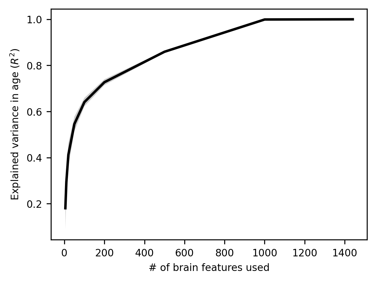
At first glance, this might look great: performance improves rapidly with the number of features, and by the time we’re sampling 1,000 features, we can predict age perfectly! But a truism in machine learning (and in life more generally) is that if something seems too good to be true, it probably is.

In this case, a bit of reflection on the fact that our model seems able to predict age with zero error should set off all kinds of alarm bells, because, on any reasonable understanding of how the world works, such a thing should be impossible. Set aside the brain data for a moment and just think about the problem of measuring chronological age. Is it plausible to think that, in a sample of over 1,000 people, including many young children and older adults, not a single person’s age would be measured with even the slightest bit of error? Remember, any measurement error should reduce our linear regression model’s performance because measurement error is irreducible. If an ABIDE-II participant’s birth date happened to be recorded as 1971 when it’s really 1961 (oops, typo!), it’s not as if our linear regression model can somehow learn to go back in time and adjust for that error.

Then think about the complexity of the brain-derived features we’re using; how well (or poorly) those features are measured/extracted; how simple our linear regression model is; and how much opportunity there is for all kinds of data quality problems to arise (is it plausible to think that all subjects’ scans are of good enough quality to extract near-perfect features?). If you spend a couple of minutes thinking along these lines, it should become very clear that an \(R^2\) of 1.0 for a problem like this is just not remotely believable. There must be something very wrong with our model. And there is: our model is overfitting our data. Because we have a lot of features to work with – even more than samples, our linear regression model is, in a sense getting creative: it’s finding all kinds of patterns in the data that look like they’re there but aren’t. We’ll spend the rest of this section exploring this idea and unpacking its momentous implications.

19.1. Understanding overfitting¶

To better understand overfitting, let’s set aside our relatively complex neuroimaging dataset for the moment and work with some simpler examples.

Let’s start by sampling some data from a noisy function where the underlying functional form is quadratic. We’ll create a small function for the data generation so that we can reuse this code later on.

def make_xy(n, sd=0.5):
    ''' Generate x and y variables from a fixed quadratic function,
    adding noise. '''
    x = np.random.normal(size=n)
    y = (0.7 * x) ** 2 + 0.1 * x + np.random.normal(10, sd, size=n)
    return x, y

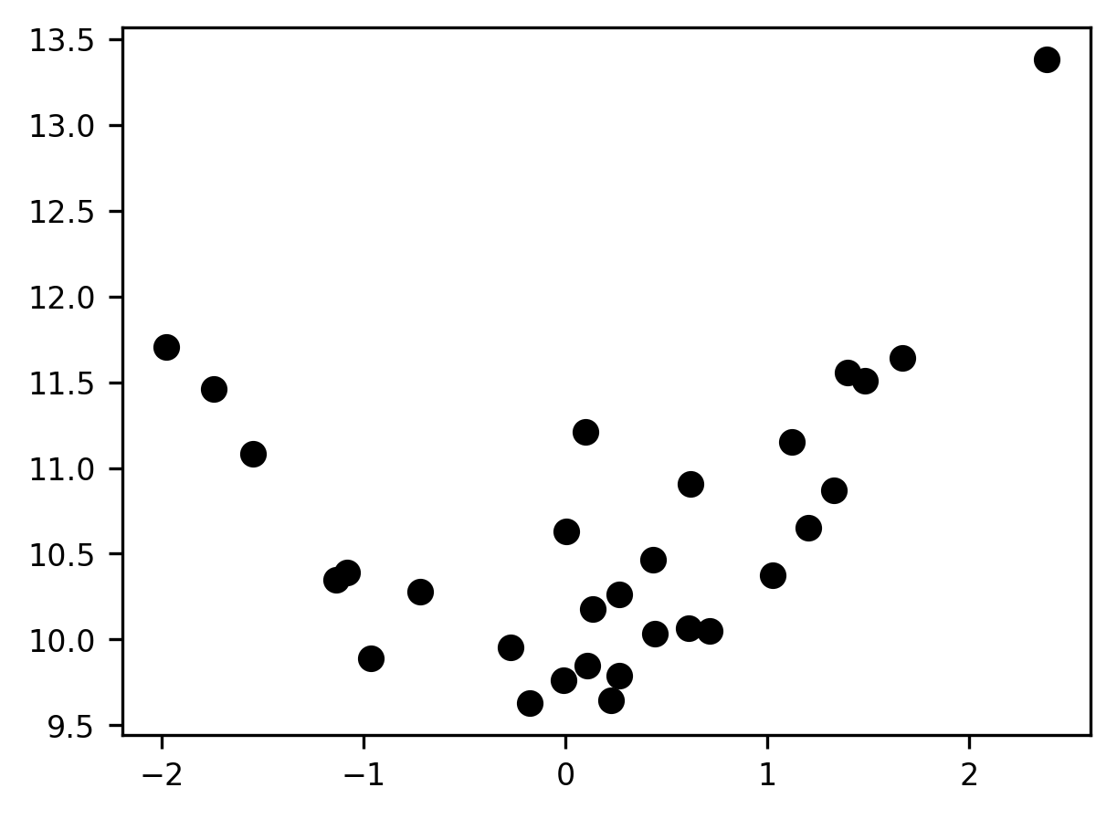
We fix the seed for the generation of random numbers and then produce some data and visualize it.

np.random.seed(10)

x, y = make_xy(30)

fig, ax = plt.subplots()
p = ax.scatter(x, y)

19.1.1. Fitting data with models of different flexibility¶

Now let’s fit that data with a linear model. To visualize the results of the linear model, we will use the model that has been fit to the data to predict the values of a range of values similar to the values of x.

from sklearn.metrics import mean_squared_error

est = LinearRegression()
est.fit(x[:, None], y)

x_range = np.linspace(x.min(), x.max(), 100)
reg_line = est.predict(x_range[:, None])

fig, ax = plt.subplots()
ax.scatter(x, y)
ax.plot(x_range, reg_line);
mse = mean_squared_error(y, est.predict(x[:, None]))
ax.set_title(f"Mean squared error: {mse:.2f}");

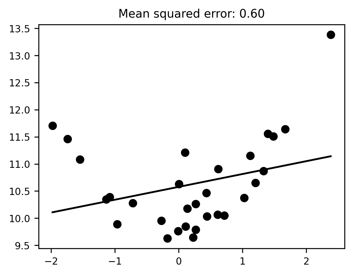
The fit looks… meh. It seems pretty clear that our linear regression model is underfitting the data—meaning, there are clear patterns in the data that the fitted model fails to describe.

What can we do about this? Well, the problem here is that our model is insufficiently flexible; our straight regression line can’t bend itself to fit the contours of the observed data. The solution is to use a more flexible estimator! A linear fit won’t cut it —- we need to fit curves.

Just to make sure we don’t underfit again, let’s use a much more flexible estimator -— specifically, a 10th-degree polynomial regression model.

This is also a good opportunity to introduce a helpful object in Scikit-learn called a Pipeline. The idea behind a Pipeline is that we can stack several transformation steps together in a sequence, and then cap them off with an Estimator of our choice. The whole pipeline will then behave like a single Estimator – i.e., we only need to call fit() and predict() once.

Using a pipeline will allow us to introduce a preprocessing step before the LinearRegression model receives our data, in which we create a bunch of polynomial features (by taking \(x^2\), \(x^3\), \(x^4\), and so on—all the way up to \(x^{10}\)). We’ll make use of Scikit Learn’s handy PolynomialFeatures transformer, which is implemented in the preprocessing module.

We’ll create a function that wraps the code to generate the pipeline, so that we can reuse that as well.

from sklearn.preprocessing import PolynomialFeatures
from sklearn.pipeline import Pipeline

def make_pipeline(degree=1):
    """Construct a Scikit Learn Pipeline with polynomial features and linear regression """
    polynomial_features = PolynomialFeatures(degree=degree, include_bias=False)

    pipeline = Pipeline([
        ("polynomial_features", polynomial_features),
        ("linear_regression", LinearRegression())
    ])
    return pipeline

Now we can initialize a pipeline with degree=10, and fit it to our toy data:

degree = 10
pipeline = make_pipeline(degree)
pipeline.fit(x[:, None], y)
reg_line = pipeline.predict(x_range[:, None])

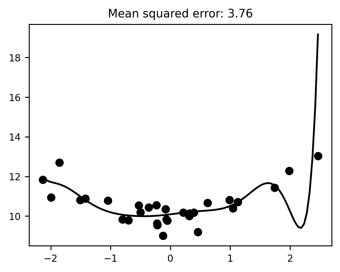
fig, ax = plt.subplots()
ax.scatter(x, y)
ax.plot(x_range, reg_line)
mse = mean_squared_error(y, pipeline.predict(x[:, None]))
ax.set_title(f"Mean squared error: {mse:.2f}");

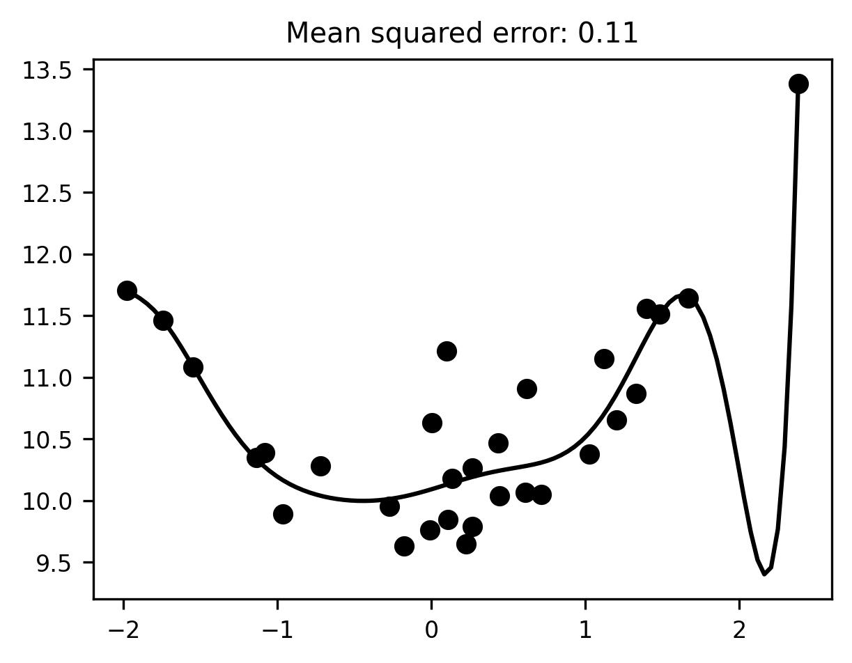
At first blush, this model seems to fit the data much better than the first model, in the sense that it reduces the mean squared error considerably relative to the simpler linear model (our MSE went down from 0.6 to 0.11). But, much as it seemed clear that the previous model was underfitting, it should now be intuitively obvious that the 10th-degree polynomial model is overfitting. The line of best fit plotted above has to bend in some fairly unnatural ways to capture individual data points. While this helps reduce the error for these particular data, it’s hard to imagine that the same line would still be very close to the data if we sampled from the same distribution a second or third time.

We can test this intuition by doing exactly that: we sample some more data from the same process and see how well our fitted model predicts the new scores.

test_x, test_y = make_xy(30)

x_range = np.linspace(test_x.min(), test_x.max(), 100)
reg_line = pipeline.predict(x_range[:, None])

fig, ax = plt.subplots()
ax.scatter(test_x, test_y)
ax.plot(x_range, reg_line)

mse = mean_squared_error(y, pipeline.predict(test_x[:, None]))
ax.set_title(f"Mean squared error: {mse:.2f}");

That’s… not good. When we apply our overfitted model to new data, the mean squared error skyrockets. The model performs significantly worse than even our underfitting linear model did.

19.1.1.1. Exercise¶

Apply the linear model to new data in the same manner. Does the linear model’s error also increase when applied to new data? Is this increase smaller or larger than what we observe for our 10th-order polynomial model?

Of course, since we wrote the data-generating process ourselves, and hence know the ground truth, we may as well go ahead and fit the data with the true functional form, which in this case is a polynomial with degree 2:

degree = 2
pipeline = make_pipeline(degree)
pipeline.fit(x[:, None], y)
x_range = np.linspace(x.min(), x.max(), 100)
reg_line = pipeline.predict(x_range[:, None])

fig, ax = plt.subplots()
ax.scatter(x, y)
ax.plot(x_range, reg_line)
mse = mean_squared_error(y, pipeline.predict(x[:, None]))
ax.set_title(f"Mean squared error: {mse:.2f}");

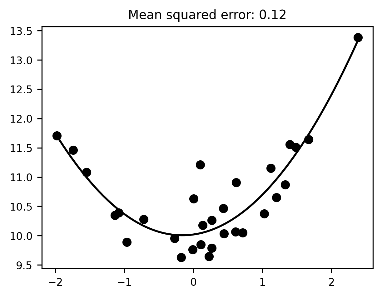
There, that looks much better. Unfortunately, in the real world, we don’t usually know the ground truth. If we did, we wouldn’t have to fit a model in the first place! So we’re forced to navigate between the two extremes of overfitting and underfitting in some other way. Finding this delicate balance is one of the central problems of machine learning -— perhaps the central problem. For any given dataset, a more flexible model will be able to capture more nuanced, subtle patterns in the data. The cost of flexibility, however, is that such a model is also more likely to fit patterns in the data that are only there because of noise, and hence won’t generalize to new samples. Conversely, a less flexible model is only capable of capturing simple patterns in the data. This means it will avoid chasing down rabbit holes full of spurious patterns, but it does so at the cost of missing out on a lot of real patterns too.

One way to think about this is that, as a data scientist, the choice you face is seldom between good models and bad ones. but rather, between lazy and energetic ones (later on, we’ll also see that there are many different ways to be lazy or energetic). The simple linear model we started with is relatively lazy: it has only one degree of freedom to play with.

The 10th-degree polynomial, by contrast, is hyperactive and sees patterns everywhere, and if it has to go very far out of its way to fit a data point that’s giving it particular trouble, it’ll happily do that.

Getting it right in any given situation requires you to strike a balance between these two extremes. Unfortunately, the precise point of optimality varies on a case-by-case basis. Later on, we’ll connect the ideas of overfitting vs. underfitting (or, relatedly, flexibility vs. stability) to another key concept -— the bias-variance tradeoff. But first, let’s turn our attention next to some of the core methods machine learners use to diagnose and prevent overfitting.

19.1.2. Additional resources¶

In case you are wondering whether overfitting happens in real research you should read the paper “I tried a bunch of things: The dangers of unexpected overfitting in classification of brain data” by Mahan Hosseini and colleagues [Hosseini et al., 2020]. It nicely demonstrates how easy it is to fall into the trap of overfitting when doing data analysis on large complex datasets, and offers some rigorous approaches to help mitigate this risk.

Neuroimaging and Data Science

Overfitting

Contents

19. Overfitting¶

19.1. Understanding overfitting¶

19.1.1. Fitting data with models of different flexibility¶

19.1.1.1. Exercise¶

19.1.2. Additional resources¶