The core concepts of machine learning
Contents
17. The core concepts of machine learning
We’ve arrived at the last chapter of the book. Hopefully you’ve enjoyed the journey to this point! In this chapter, we’ll dive into machine learning. There’s a lot to cover, so this will be a pretty long chapter. To keep things manageable, we’ve structured the material into 7 sections. Here in Section 17, we’ll review some core concepts in machine learning, setting the stage for everything that follows. In Section 18, we’ll introduce the Scikit-learn Python package, which we’ll rely on heavily throughout the chapter. Section 19 explores the central problem of overfitting; Section 20 and Section 21 then cover different ways of diagnosing and addressing overfitting via model validation and model selection, respectively. Finally, in Section 22, we close with a brief review of deep learning methods -— a branch of machine learning that has made many recent advances, and one that’s recently made considerable inroads into neuroimaging.
Before we get into it, a quick word about our guiding philosophy. Many texts covering machine learning adopt what we might call a “catalog” approach: they try to cover as many of the different classes of machine learning algorithms as possible. This won’t be our approach here. For one thing, there’s simply no way to do justice to even a small fraction of this space within the confines of one chapter (even a long one). More importantly, though, we think it’s far more important to develop a basic grasp on core concepts and tools in machine learning than to have a cursory familiarity with many of the different algorithms out there. In our anecdotal experience, neuroimaging researchers new to machine learning are often bewildered by the sheer number of algorithms implemented in machine learning packages like Scikit-learn, and sometimes fall into the trap of systematically applying every available algorithm to their problem, in the hopes of identifying the “best” one. For reasons we’ll discuss in depth in this chapter, this kind of approach can be quite dangerous; not only does it preempt a deeper understanding of what one is doing, but, as we’ll see in Section 19 and Section 20, it can make one’s results considerably worse by increasing the risk of overfitting.
17.1. What is machine learning?
This is a chapter on machine learning, so now is probably a good time to give a working definition. Here’s a reasonable one: machine learning is the field of science/engineering that seeks to build systems capable of learning from experience.
This is a very broad definition, and in practice, the set of activities that get labeled “machine learning” is quite broad and varied. But two elements are common to most machine learning applications: (1) an emphasis is on developing algorithms that can learn (semi-)autonomously from data, rather than static rule-based systems that must be explicitly designed or updated by humans; and (2) an approach to performance evaluation that focuses heavily on well-defined quantitative targets.
We can contrast machine learning with traditional scientific inference, where the goal (or at least, a goal) is to understand or explain how a system operates.
The goals of prediction and explanation are not mutually exclusive, of course. But most people tend to favor one over the other to some extent. And, as a rough generalization, people who do machine learning tend to be more interested in figuring out how to make useful predictions than in arriving at a “true”, or even just an approximately correct, model of the data-generating process underlying a given phenomenon. By contrast, people interested in explanation might be willing to accept models that don’t make the strongest possible predictions (or often, even good ones) so long as those models provide some insight into the mechanisms that seem to underlie the data.
We don’t need to take a principled position on the prediction vs. explanation divide here (plenty has been written on the topic; see Section 17.4.3 below). Just be aware that, for purposes of this chapter, we’re going to assume that our goal is mainly to generate good predictions, and that understanding and interpretability are secondary or tertiary on our list of desiderata (though we’ll still say something about them now and then).
17.2. Supervised vs. unsupervised learning
Broadly speaking, machine learning can be carved up into two forms of learning:
supervised and unsupervised. We say that learning is supervised whenever
we know the true values that our model is trying to predict, and hence, are in a
position to “supervise” the learning process by quantifying prediction accuracy
and the associated prediction error. “Ordinary” least-squares regression, in the
machine learning context, is an example of supervised learning: our model takes
as its input both a vector of features (conventionally labeled X) and a
vector of labels (y). Researchers often use different terminology in various
biomedical disciplines—often calling X variables or predictors, and y
the outcome or dependent variable—but the idea is the same.
Here are some examples of supervised learning problems (the first of which we’ll attempt later):
Predicting people’s chronological age from structural brain differences
Determining whether or not an incoming email is spam
Predicting a person’s rating of a particular movie based on their ratings of other movies
Discriminating schizophrenics from controls based on genetic markers
In each of these cases, we expect to train our model using a dataset where we know the ground truth—i.e., we have labeled examples of age, spam, movie ratings, and a schizophrenia diagnosis, in addition to any number of potential features we might use to try and predict each of these labels.
17.3. Supervised learning: classification vs. regression
Within the class of supervised learning problems, we can draw a further distinction between classification problems and regression problems. In both cases, the goal is to develop a predictive model that recovers the true labels as accurately as possible. The difference between the two lies in the nature of the labels: in classification, the labels reflect discrete classes; in regression, the labeled values vary continuously.
17.3.1. Regression
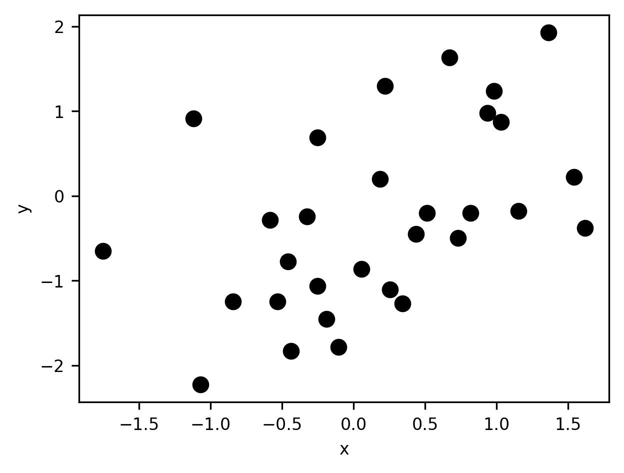
A regression problem arises any time we have a set of continuous numerical labels and we’re interested in using one or more features to try and predict those labels. Any bivariate relationship can be conceptualized as a regression of one variable on the other. For example, suppose we have the data displayed in this scatterplot:
import numpy as np
import matplotlib.pyplot as plt
x = np.random.normal(size=30)
y = x * 0.5 + np.random.normal(size=30)

fig, ax = plt.subplots()
ax.scatter(x, y, s=50)
ax.set_xlabel('x')
label = ax.set_ylabel('y')
We can frame this as a regression problem by saying that our goal is to generate
the best possible prediction for y given knowledge of x. There are many ways
to define what constitutes the “best” prediction, but here we’ll use the
least-squares criterion and say we want a model that, when given the x
scores as inputs, will produce predictions for y that minimize the sum of
squared deviations between the predicted scores and the true scores.
This is what “ordinary” least-squares (OLS) regression gives us. Here’s the OLS
solution: first we add a column to x. This column will be used to model the
intercept of the line that relates y to x.
x_with_int = np.hstack((np.ones((len(x), 1)), x[:, None]))
Then, we solve the set of linear equations using Scipy’s linear algebra routines. This gives us parameter estimates for the intercept and the slope.
w = np.linalg.lstsq(x_with_int, y, rcond=None)[0]
print("Parameter estimates (intercept and slope):", w)
Parameter estimates (intercept and slope): [-0.36822492 0.62140416]
Then, we visualize the data and also a straight line that represents the model of the data based on the regression:
fig, ax = plt.subplots()
ax.scatter(x, y, s=50)
ax.set_xlabel('x')
ax.set_ylabel('y')

xx = np.linspace(x.min(), x.max()).T
line = w[0] + w[1] * xx

p = plt.plot(xx, line)
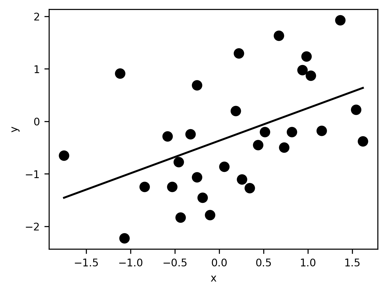
What is this model? Based on the values of the parameters, we can say that the linear prediction equation that produced the predicted scores above can be written as \(\hat{y} = -0.37 + 0.62x\).
Of course, not every model we use to generate a prediction will be quite this simple. Most won’t—either because they have more parameters, or because the prediction can’t be expressed as a simple weighted sum of the parameter values. But what all regression problems share in common with this very simple example is the use of one or more features to try and predict labels that vary continuously.
17.3.2. Classification
Classification problems are conceptually similar to regression problems. In classification, just like in regression, we’re still trying to learn to make the best predictions we can for some target set of labels. The difference is that the labels are now discrete rather than continuous. In the simplest case, the labels are binary: there are only two classes. For example, we can use utilities from the Scikit Learn library (we’ll learn more about this library in Section 18) to create data that look like this
from sklearn.datasets import make_blobs

X, y = make_blobs(centers=2, random_state=2)
fig, ax = plt.subplots()
s = ax.scatter(*X.T, c=y, s=60, edgecolor='k', linewidth=1)
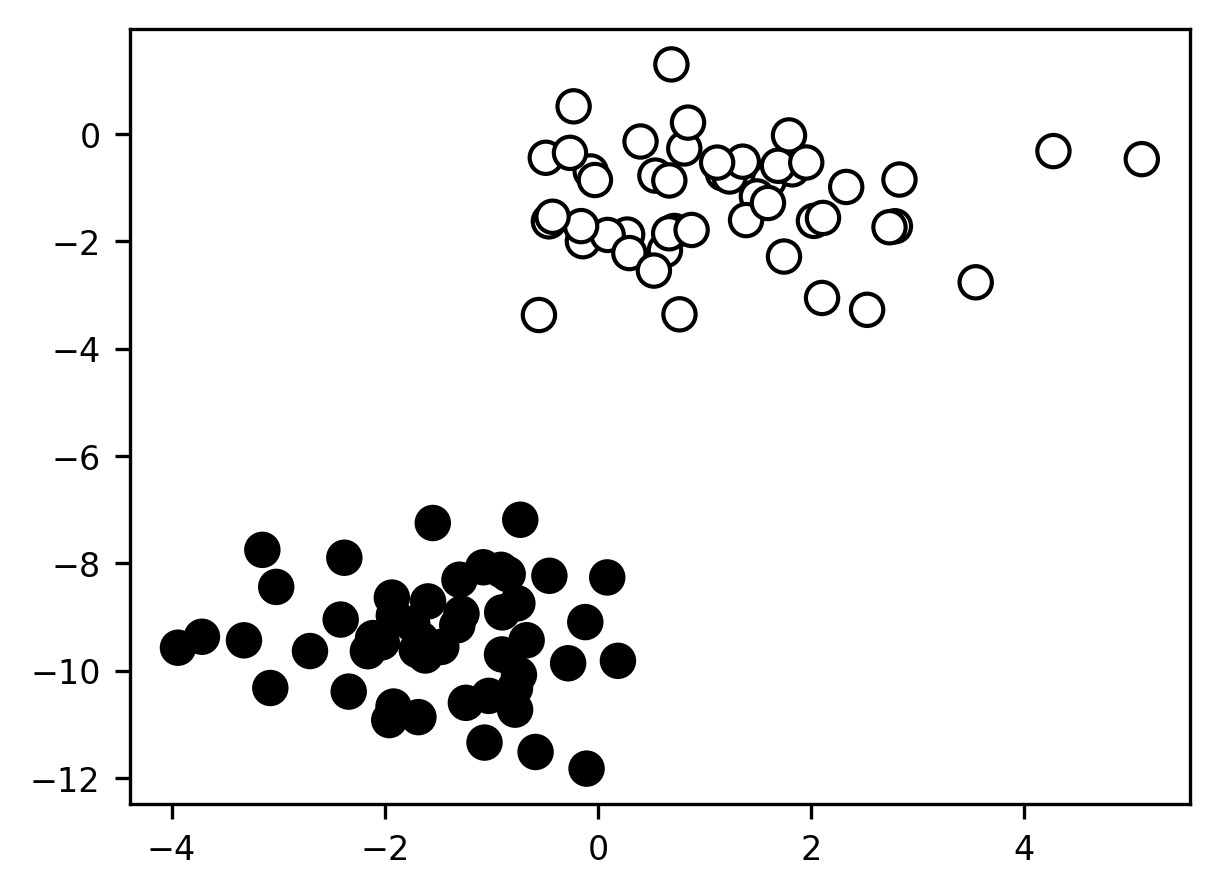
Here, we have two features (on the x- and y-axes) we can use to try to correctly classify each sample. The two classes are labeled by color.
In the above example, the classification problem is quite trivial: it’s clear to the eye that the two classes are perfectly linearly separable so that we can correctly classify 100% of the samples just by drawing a line between them. Of course, most real-world problems won’t be nearly this simple. As we’ll see later, when we work with real data, the feature-space distributions of our labeled cases will usually overlap considerably, so that no single feature (and often, not even all of our features collectively) will be sufficient to perfectly discriminate cases in each class from cases in other classes.
17.4. Unsupervised learning: clustering and dimensionality reduction
In unsupervised learning, we don’t know the ground truth. We have a dataset
containing some observations that vary on some set of features X, but we’re
not given any set of accompanying labels y that we’re supposed to try to
recover using X. Instead, the goal of unsupervised learning is to find
interesting or useful structure in the data. What counts as interesting or
useful is of course very much person and context-dependent. But the key point is
that there is no strictly right or wrong way to organize our samples (or if
there is, we don’t have access to that knowledge). So we’re forced to muddle
along the best we can, using only the variation in the X features to try and
make sense of our data in ways that we think might be helpful to us later.
Broadly speaking, we can categorize unsupervised learning applications into two classes: clustering and dimensionality reduction.
17.4.1. Clustering
In clustering, our goal is to label the samples we have into discrete clusters (or groups). In a sense, clustering is just classification without ground truth. In classification, we’re trying to recover the class assignments that we know to be there; in clustering, we’re trying to make class assignments even though we have no idea what the classes truly are, or even if they exist at all.
The best-case scenario for a clustering application might look something like this:
X, y = make_blobs(random_state=100)
fig, ax = plt.subplots()
s = ax.scatter(*X.T)
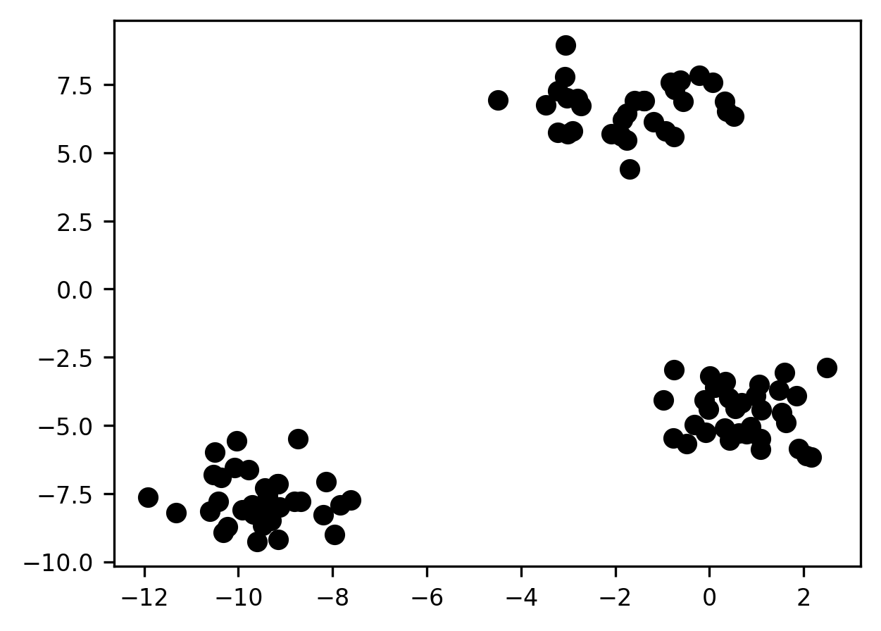
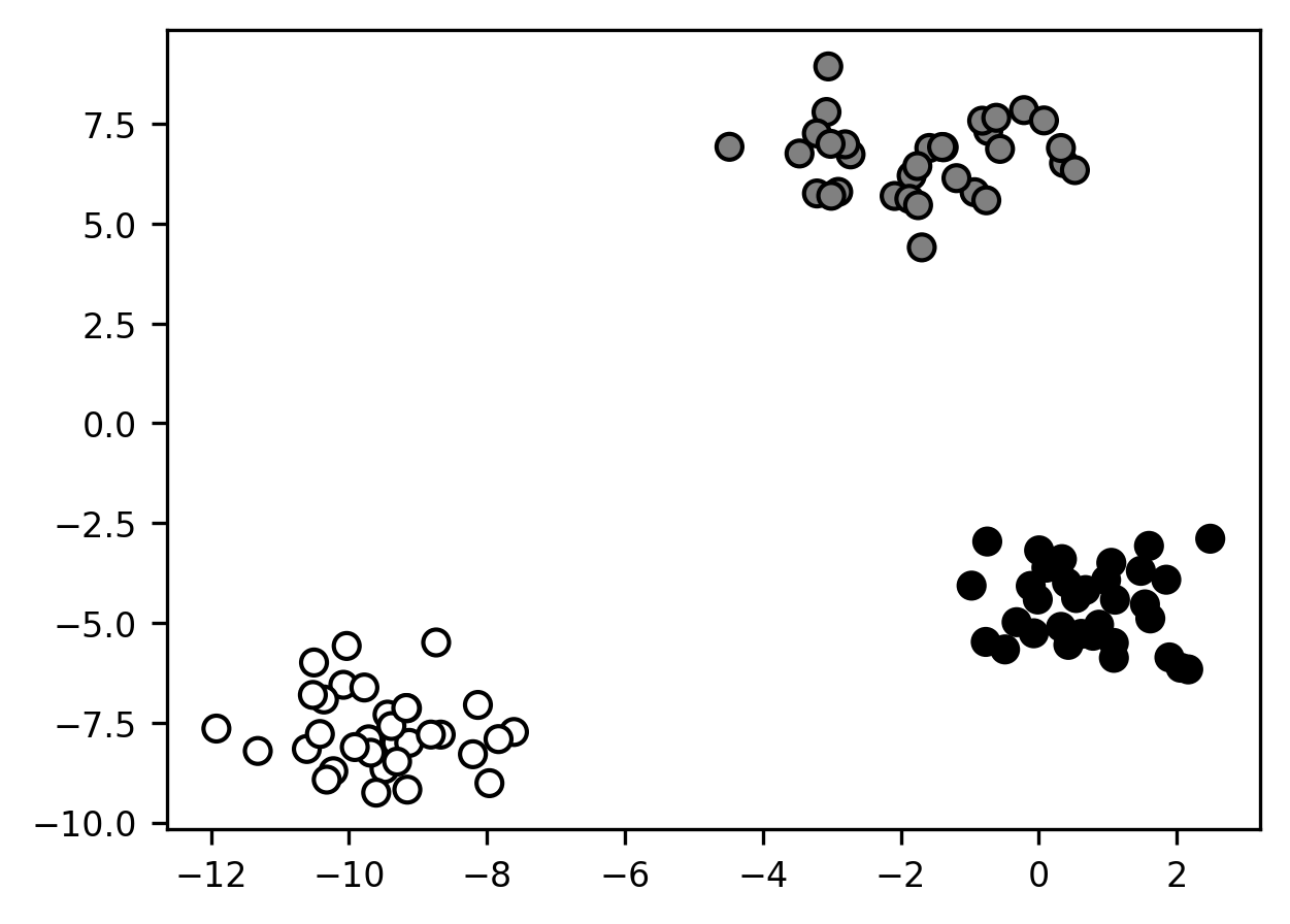
Remember: we don’t know the true labels for these observations (that’s why they’re all assigned the same color in the above plot). So in a sense, any cluster assignment we come up with is just our best guess as to what might be going on. Nevertheless, in this particular case, the spatial grouping of the samples in 2 dimensions is so striking that it’s hard to imagine us having any confidence in any assignment except the following one:
X, y = make_blobs(random_state=100)
fig, ax = plt.subplots()
s = ax.scatter(*X.T, c=y)
Of course, just as with the toy classification problem we saw earlier, clustering problems this neat rarely show up in nature. Worse, in the real world, there often aren’t any “true” clusters. Often, the underlying data-generating process is best understood as a complex (i.e., high-dimensional) continuous function. In such cases, clustering can still be very helpful, as it can help reduce complexity and give us insight into regularities in the data. But when we use clustering methods (and, more generally, any kind of unsupervised learning approach), we should try to always remember the adage that the map is not the territory—meaning, we shouldn’t mistake a description of a phenomenon for the phenomenon itself.
17.4.2. Dimensionality reduction
The other major class of unsupervised learning application is dimensionality reduction. Here, the idea, just as the name suggests, is to reduce the dimensionality of our data. The reasons why dimensionality reduction is important in machine learning will become clearer when we talk about overfitting later, but a general intuition we can build on is that most real-world datasets—especially large ones—can be efficiently described using fewer dimensions than there are nominal features in the dataset. Real-world datasets tend to contain a good deal of structure: variables are related to one another in important (though often non-trivial) ways, and some variables are redundant with others, in the sense that they can be redescribed as functions of other variables. The idea is that, if we can capture most of the variation in the features of a dataset using a smaller subset of those features, we can reduce the effective size of our dataset and build predictions more efficiently.
To illustrate, consider this dataset:
x = np.random.normal(size=300)
y = x * 5 + np.random.normal(size=300)

fig, ax = plt.subplots()
s = ax.scatter(x, y)

Nominally, this is a two-dimensional dataset, and we’re plotting the two features on the x and y axes, respectively. But it seems clear at a glance that there aren’t really two dimensions in the data—or at the very least, one dimension is far more important than the other. In this case, we could capture the vast majority of the variance along both dimensions with a single axis placed along the diagonal of the plot—in essence, “rotating” the axes to a “simpler” structure. If we keep only the first dimension in the new space and lose the second dimension, we reduce our 2-dimensional dataset to 1 dimension, with very little loss of information. In the next section, we will dive into the nuts and bolts of machine learning in Python, by introducing the Scikit Learn machine learning library.
17.4.3. Additional resources
If you are interested in diving deeper into the distinction between prediction and explanation, we really recommend Leo Breiman’s classical paper “The two cultures of statistical modeling” [Breiman, 2001] . Another great paper on this topic is Galit Shmueli’s “To explain or to predict?” [Shmueli, 2010]. Finally you can read one of us weighing in on the topic, together with Jake Westfall, in a paper titled “Choosing Prediction Over Explanation in Psychology: Lessons From Machine Learning” [Yarkoni and Westfall, 2017].