Image segmentation
Contents
15. Image segmentation
The general scope of image processing and some basic terminology were introduced in Section 14. We will now dive deeper into specific image processing methods in a bit more detail. We are going to look at computational tasks that are in common use in neuroimaging data analysis and we are going to demonstrate some solutions to these problems using relatively simple computations.
The first is image segmentation. Image segmentation divides the pixels or voxels of an image into different groups. For example, you might divide a neuroimaging dataset into parts that contain the brain itself and parts that are non-brain (e.g., background, skull, etc.). Generally speaking, segmenting an image allows us to know where different objects are in an image and allows us to separately analyze parts of the image that contain particular objects of interest. Let’s look at a specific example. We’ll start by loading a neuroimaging dataset that has BOLD fMRI images in it:
from ndslib import load_data
brain = load_data("bold_volume")
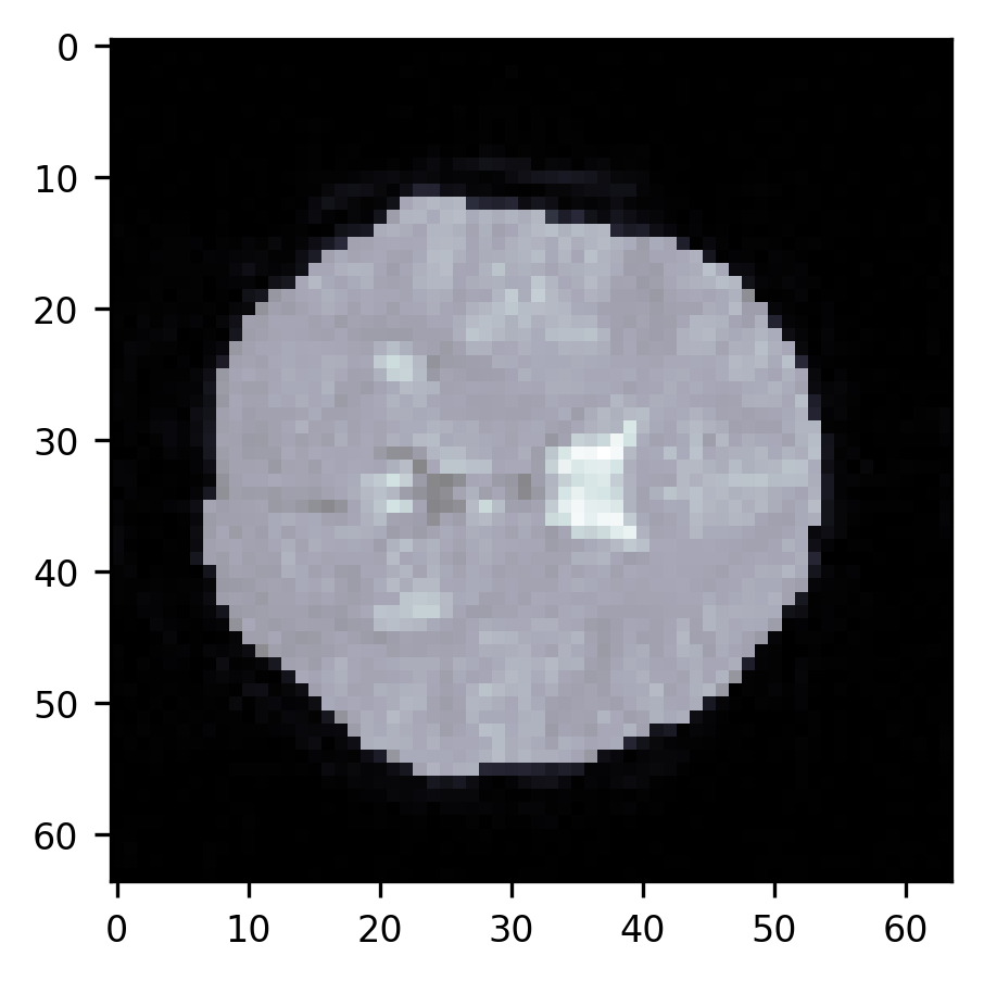
For simplicity’s sake, we will look only at one slice of the data for now. Let’s take a horizontal slice roughly in the middle of the brain. Visualizing the image can help us understand the challenges that segmentation helps us tackle.
slice10 = brain[:, :, 10]
import matplotlib.pyplot as plt
fig, ax = plt.subplots()
im = ax.imshow(slice10, cmap="bone")
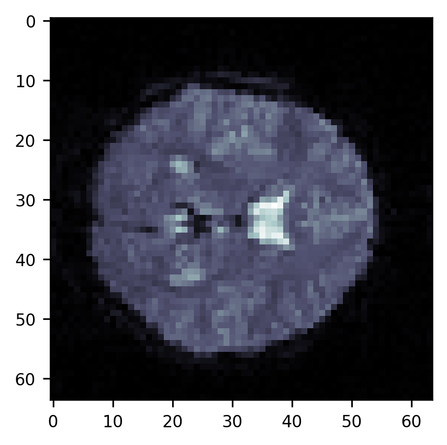
First of all, a large part of the image is in the background – the air around the subject’s head. If we are going to do statistical computations on the data in each of the voxels, we would like to avoid looking at these voxels. That would be a waste of time. In addition, there are parts of the image that are not clearly in the background but contain parts of the subject’s head or parts of the brain that we are not interested in. For example, we don’t want to analyze the voxels that contain parts of the subject’s skull and/or skin that appear as bright lines alongside the top of the part of the image that contains the brain. We also don’t want to analyze the voxels that are in the ventricles, appearing here as brighter parts of the image. To be able to select only the voxels that are in the brain proper, we need to segment the image into brain and non-brain. There are a few different approaches to this problem.
15.1. Intensity-based segmentation
The first and simplest approach to segmentation is to use the distribution of pixel intensities as a basis for segmentation As you can see, the parts of the image that contain the brain are brighter – have higher intensity values. The parts of the image that contain the background are dark and contain low-intensity values. One way of looking at the intensity values in the image is using a histogram. This code displays a histogram of pixel intensity values. I am using the Matplotlib “hist” function, which expects a one-dimensional array as input, so the input is the “flat” representation of the image array, which unfolds the two-dimensional array into a one-dimensional array.
fig, ax = plt.subplots()
p = ax.hist(slice10.flat)
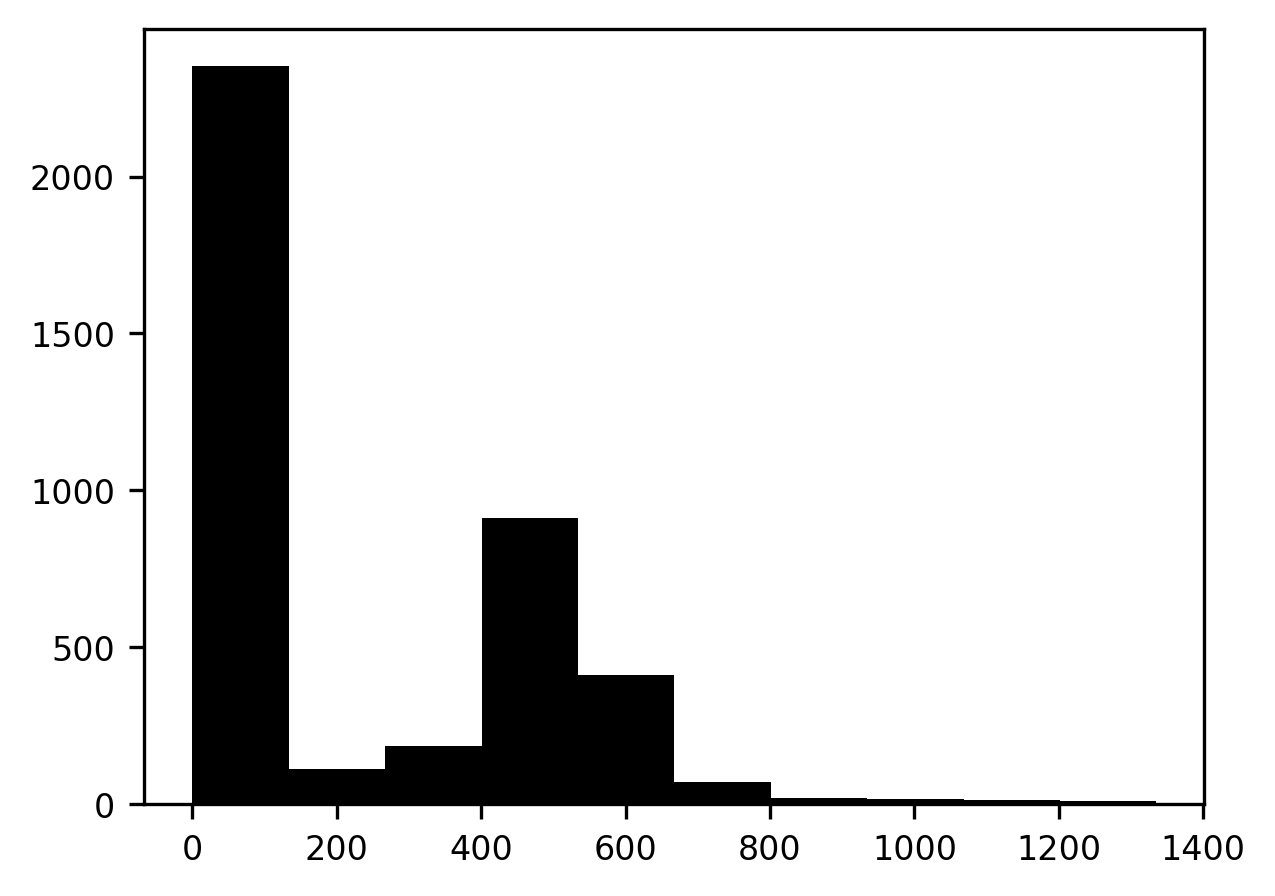
The histogram has two peaks. A peak at lower pixel intensity values, close to 0, corresponds to the dark part of the image that contains the background, and a peak at higher intensity values, corresponds to the bright part of the image that contains the brain
One approach to segmentation would be to find a threshold value. Pixels with values below this threshold would be assigned to the background and values equal to or above this threshold would be assigned to the brain
For example, we can select the mean pixel intensity to be our threshold. Here, I am displaying the image intensity histogram, together with the mean value, represented as a vertical dashed line. What would a segmentation based on this value look like?
import numpy as np
mean = np.mean(slice10)
fig, ax = plt.subplots()
ax.hist(slice10.flat)
p = ax.axvline(mean, linestyle='dashed')

We start by creating a segmentation image that contains all zeros. Using Boolean indexing, we select those parts of the segmentation image that correspond to parts of the brain image that have intensities higher than the threshold and set these to 1 (see also Section 8.2.8). Then, we can display this image on top of our brain image. To make sure that we can see the brain image through the segmentation image, we set it to be slightly transparent. This is done by setting an imaging parameter called “alpha”, which describes the opacity of an image (where 0 is fully transparent and 1.0 is fully opaque) to 0.5. This lets us see how well the segmentation overlaps with the brain image.
segmentation = np.zeros_like(slice10)
segmentation[slice10 > mean] = 1

fig, ax = plt.subplots()
ax.imshow(slice10, cmap="bone")
im = ax.imshow(segmentation, alpha=0.5)
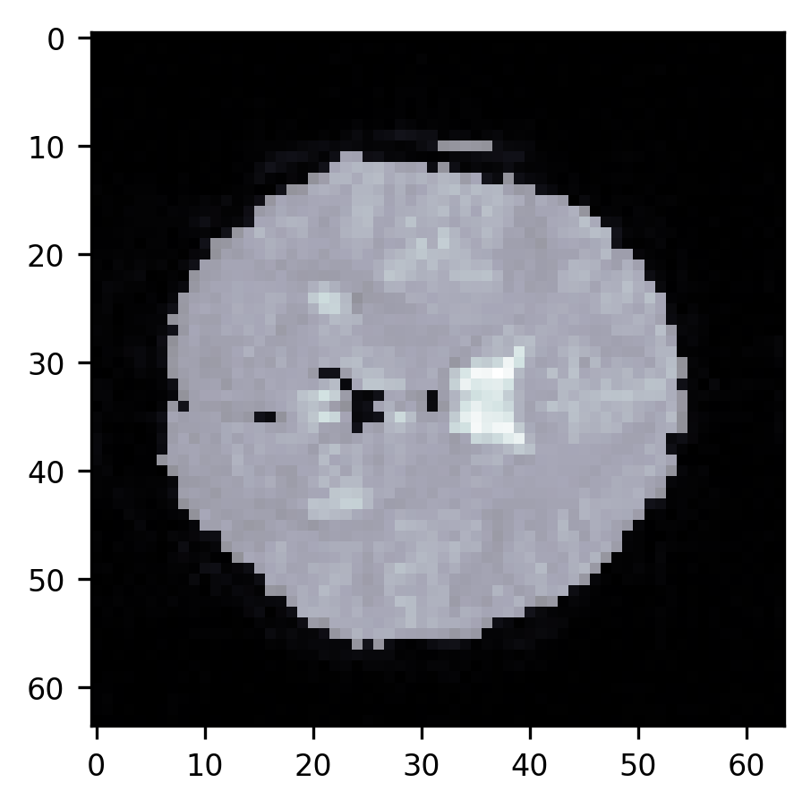
With this visualization, we can see the brain through the transparency of the segmentation mask. We can see that the mean threshold is already pretty effective at segmenting out parts of the image that contain the background, but there are still parts of the image that should belong to the background and are still considered to be part of the brain. In particular, parts of the skull and the dura mater get associated with the brain, because they appear bright in the image. Also, the ventricles, which appear brighter in this image, are classified as part of the brain. The challenge is to find a value of the threshold that gives us a better segmentation.
15.1.1. Otsu’s method
A classic approach to this problem is now known as “Otsu’s method”, after the Japanese engineer Nobuyuki Otsu, who invented it in the 1970s [Otsu, 1979]. The method relies on a straightforward principle: find a threshold that minimizes the variance in pixel intensities within each class of pixels (for example, brain and non-brain). This principle is based on the idea that pixels within each of these segments should be as similar as possible to each other, and as different as possible from the other segment. It also turns out that this is a very effective strategy for many other cases where you would like to separate the background from the foreground (for example, text on a page).
Let’s examine this method in more detail. We are looking for a threshold that would minimize the total variance in pixel intensities within each class, or “intraclass variance”. This has two components: The first is the variance of pixel intensities in the background pixels, weighted by the proportion of the image that is in the background. The other is the variance of pixel intensities in the foreground, weighted by the proportion of pixels belonging to the foreground. To find this threshold value, Otsu’s method relies on the following procedure: Calculate the intraclass variance for every possible value of the threshold and find the candidate threshold that corresponds to the minimal intraclass variance. We will look at an example with some code below, but we will first describe this approach in even more detail with words.
We want to find a threshold corresponding to as small as possible intraclass
variance, so we start by initializing our guess of the intraclass variance to
the largest possible number: infinity. We are certain that we will find a value
of the threshold that will have a smaller intraclass variance than that. Then,
we consider each possible pixel value that could be the threshold. In this case,
that’s every unique pixel value in the image (which we find using np.unique).
As background, we select the pixel values that have values lower than the
threshold. As foreground, we select the values that have values equal to or
higher than the threshold.
Then, the foreground contribution to the intraclass variance is the variance of
the intensities among the foreground pixels (np.var(foreground), multiplied by
the number of foreground pixels (len(foreground)). The background contribution
to the intraclass variance is the variance of the intensities in the background
pixels, multiplied by the number of background pixels (with very similar code
for each of these). The intraclass variance is the sum of these two. If this
value is smaller than the previously found best intraclass variance, we set this
to be the new bests intraclass variance, and replace our previously found
threshold with this one. After running through all the candidates, the value
stored in the threshold variable will be the value of the candidate that
corresponds to the smallest possible intraclass variance.
This is the value that you would use to segment the image. Let’s look at the implementation of this algorithm
min_intraclass_variance = np.inf

for candidate in np.unique(slice10):
    foreground = slice10[slice10 < candidate]
    background = slice10[slice10 >= candidate]
    if len(foreground) and len(background):
        foreground_variance = np.var(foreground) * len(foreground)
        background_variance =  np.var(background) * len(background)
        intraclass_variance = foreground_variance + background_variance
        if intraclass_variance < min_intraclass_variance:
            min_intraclass_variance = intraclass_variance
            threshold = candidate
Having run through this, let’s see if we found something different from our previous guess – the mean of the pixel values. We add this value to the histogram of pixel values as a dotted line. It looks like the value that Otsu’s method finds is a bit higher than the mean pixel value.
mean = np.mean(slice10)
fig, ax = plt.subplots()
ax.hist(slice10.flat)
ax.axvline(mean, linestyle='dashed')
p = ax.axvline(threshold, linestyle='dotted')

How well does this segmentation strategy work?
We’ll use the same code we used before, creating an array of zeros, and replacing the zeros with ones only in those parts of the array that correspond to pixels in the image that have values smaller than the threshold.
segmentation = np.zeros_like(slice10)
segmentation[slice10 > threshold] = 1

fig, ax = plt.subplots()
ax.imshow(slice10, cmap="bone")
p = ax.imshow(segmentation, alpha=0.5)
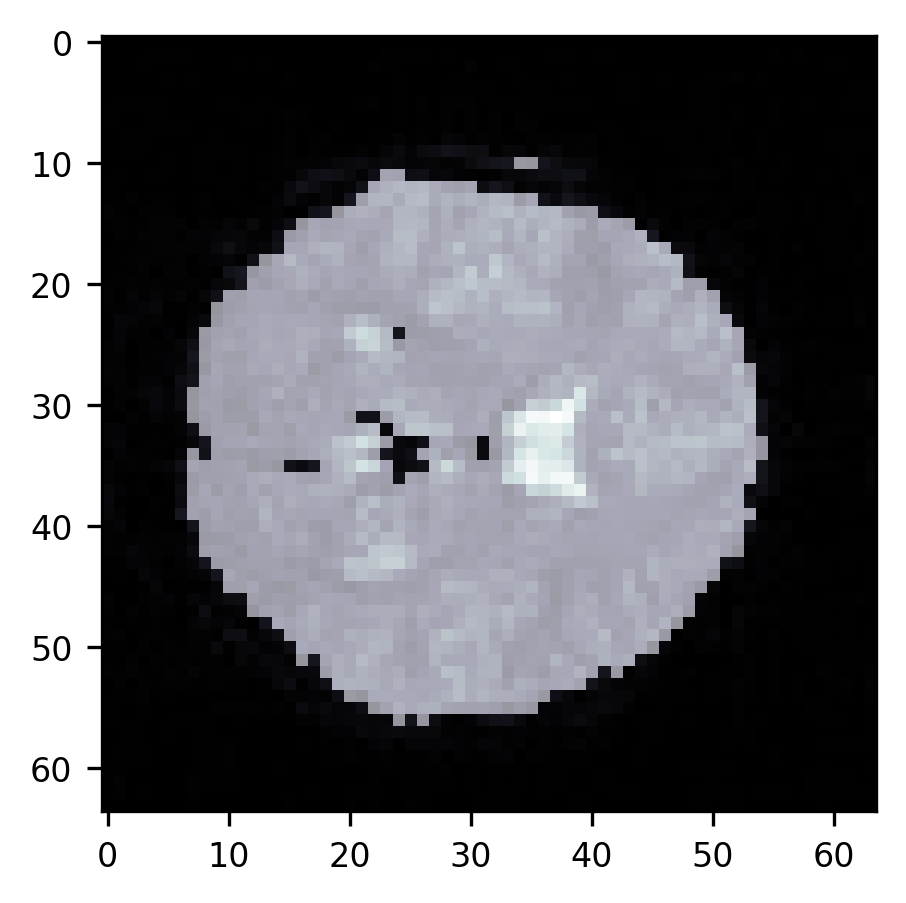
As you can see, this segmentation is quite good. There are almost no more voxels
outside the brain that are misclassified as being in the brain. We still have
trouble with the ventricles, though. This highlights the limitation of this
method. In particular, a single threshold may not be enough. In the exercise
below, you will be asked to think about this problem more, but before we move on
and talk about other approaches to segmentation, we’ll just point out that if
you do want to use Otsu’s method for anything, you should probably use the
Scikit Image implementation of it, which is in skimage.filters.threshold_otsu.
It’s much faster and more robust than the simple implementation we outlined
above. If you want to learn more about how to speed up slow code, reading
through the source code of this function 1 is an interesting case study.
15.1.1.1. Exercises
Using the code that we implemented above, implement code that finds two threshold values to segment the brain slice into three different segments. Does this adequately separate the ventricles from other brain tissue based on their intensity? Compare the performance of your implementation to the results of Scikit Image’s
skimage.filters.threshold_multiotsu.The
skimage.filtersmodule has a function calledtry_all_threshold, which compares several different approaches to threshold-based segmentation. Run this function to compare the methods. Which one works best on this brain image? How would you evaluate that objectively?
Image processing, computer vision and neuroscience
There has always been an interesting link between image processing and neuroscience. This is because one of the goals of computational image processing is to create algorithms that mimic operations that our eyes and brain can easily do. For example, the segmentation task that we are trying to automate in this chapter is one that our visual system can learn do with relative ease. One of the founders of contemporary computational neuroscience was David Marr. One of his main contributions to computational neuroscience was in breaking apart problems in neuroscience conceptually to three levels: computational, algorithmic and implementational. The computational level can be thought of as the purpose of the system, or the problem that the system is solving. The algorithmic level is a series of steps or operations – ideally defined mathematically – that the system can take to solve the problem. Finally, the implementation level is the specific way in which the algorithm is instantiated in the circuitry of the nervous system. This view of neuroscience has been hugely influential and has inspired both efforts to understand the nervous system based on predictions from both the computational and algorithmic levels, as well as efforts to develop algorithms that are inspired by the architecture of the brain. For example, in 1980, Marr and Ellen Hildreth wrote a paper that described the theory of edge detection and also proposed an algorithm that finds edges in images [Marr and Hildreth, 1980]. Their premise was that the computational task that is undertaken by the first few stages in the visual system is to construct a “rich but primitive description of the image”. What they called the “raw primal sketch” should provide the rest of the visual system – the parts that figure out what objects are out in the world and what they are doing – with information about things like edges, surfaces and reflectances. Based on this computational requirement, they designed an algorithm that would specialize at finding edges. This was a particular kind of filter/kernel that, when convolved with images, would find the parts of the image where edges exist. Based on some theoretical considerations they defined this kernel to be a difference of two Gaussians with two different variances. This edge detector was inspired to some degree by the operations that Marr and Hildreth knew that the early visual cortex performs. In addition, their article proposed some predictions for what operations the visual system should be doing if this is the way that it indeed performs edge detection.
15.2. Edge-based segmentation
Threshold-based segmentation assumes that different parts of the image that should belong to different segments should have different distributions of pixel values. In many cases that is true. But this approach does not take advantage of the spatial layout of the image. Another approach to segmentation uses the fact that parts of the image that should belong to different segments are usually separated by edges. What is an edge? Usually, these are contiguous boundaries between parts of the image that look different from each other. These differences can be differences in intensity, but also differences in texture, pattern, and so on. In a sense, finding edges and segmenting the image are a bit of a chicken and egg: if you knew where different parts of the image were, you wouldn’t have to segment them. Nevertheless, in practice, using algorithms that specifically focus on finding edges in the image can be useful to perform the segmentation. Finding edges in images has been an important part of computer vision for about as long as there has been a field called computer vision. As you saw in chapter Section 14, one part of finding edges could be to construct a filter that emphasizes changes in the intensity of the pixels (such as the Sobel filter that you explored in the exercise in Section 14.4.3.1). Sophisticated edge detection algorithms can use this, together with a few more steps, to more robustly find edges that extend in space. One such algorithm is the Canny edge detector, named after its inventor, John Canny, a computer scientist, and computer vision researcher [Canny, 1986]. The algorithm takes several steps that include smoothing the image to get rid of noisy or small parts, finding the local gradients of the image (for example, with the Sobel filter) and then thresholding this image, selecting edges that are connected to other strong edges and suppressing edges that are connected to weaker edges. We will not implement this algorithm step by step, but instead, use the algorithm as it is implemented in Scikit Image. If you are interested in learning more about the algorithm and would like an extra challenge, we would recommend also reading through the source code of the Scikit Image implementation 2. It’s just a few dozen lines of code, and understanding each step that the code is taking will help you understand this method much better. For now, we will use this as a black box and see whether it helps us with the segmentation problem. We start by running our image through the canny edge detector. This creates an image of the edges, containing a 1 in locations that are considered to be at an edge and 0 in all other locations.
from skimage.feature import canny
edges = canny(slice10)

fig, ax = plt.subplots()
ax.imshow(slice10, cmap="gray")
im = ax.imshow(edges, alpha=0.5)
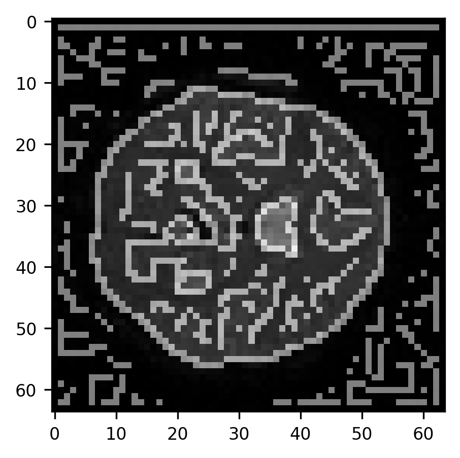
As you can see, the algorithm finds edges both around the perimeter of the brain as well as within the brain. This just shows us that the Canny algorithm is very good at overcoming one of the main challenges of edge detection, which is that edges are defined by intensity gradients across a very large range of different intensities. That is, an edge can be a large difference between very low pixel intensities (for example, between the background and the edge of the brain) as well as between very high pixel intensities (parts of the brain and the ventricles). Next, we will use some morphological operations to fill parts of the image that are enclosed within edges and to remove smaller objects that are spurious (see Section 14.4.4).
from scipy.ndimage import binary_fill_holes
from skimage.morphology import erosion, remove_small_objects
segmentation = remove_small_objects(erosion(binary_fill_holes(edges)))
fig, ax = plt.subplots()
ax.imshow(slice10, cmap="bone")
im = ax.imshow(segmentation, alpha=0.5)
This approach very effectively gets rid of the parts of the skull around the brain, but it does not separate the ventricles from the rest of the brain. It also doesn’t necessarily work as well in other slices of this brain (as an exercise, try running this sequence of commands on other slices. When does it work well? When does it fail?). Brain data segmentation is a very difficult task. Though we introduced a few approaches here, we don’t necessarily recommend that you rely on these approaches as they are. The algorithms that are used in practice to do brain segmentations rely not only on the principles that we showed here but also on knowledge of brain structure and extensive validation experiments. Segmentation of brain data into multiple structures and tissue types, as done, for example, by the popular Freesurfer software, requires such knowledge. But this does demonstrate a few of the fundamental operations that you might use if you were to start down your path of developing such algorithms for new use cases.
15.3. Additional resources
Both Nobuyuki Otsu’s original description of Otsu’s method [Otsu, 1979] and John Canny’s original description of the Canny filter [Canny, 1986] are good reads if you want to understand the use cases and development of this kind of algorithm and of image-processing pipelines more generally.