9. Manipulating tabular data with Pandas¶

As we saw in a previous chapter, many kinds of neuroscience data can be described as arrays. In particular, the analysis of many physiological signals, such as BOLD, really benefits from organizing data in the form of arrays. But there’s another very beneficial way of organizing data. In neuroscience, we often have datasets where several different variables were recorded for each observation in the dataset. For example, each observation might be one subject in a study, and for each subject, we record variables like the subject’s sex and age, various psychological measures, and also summaries of physiological measurements using fMRI or other brain imaging modalities. In cases like this, it’s very common to represent the data in a two-dimensional table where each row represents a different observation and each column represents a different variable. Organizing our data this way allows us to manipulate the data through queries and aggregation operations in a way that makes analysis much easier. Because this type of organization is so simple and useful, it’s often called “tidy” data (a more technical name, for readers with an acquaintance with databases, is the third normal form, or 3NF). This is also a very general way of organizing data in many different applications, ranging from scientific research to website logs, and administrative data collected in the operations of various organizations. As you will see later in the book, it is also a natural input to further analysis. For example, with the machine-learning methods that you will see in sklearn. For this reason, tools that analyze tidy tabular data play a central role in data science across these varied applications. Here, we’ll focus on a popular Python library that analyzes this kind of data: “Pandas”. Pandas is not only the plural form of an exceedingly cute animal you can use as the mascot for your software library but also an abbreviation of “panel data”, which is another name for data that is stored in two-dimensional tables of this sort.

An example should help demonstrate how Pandas is used. Let’s consider a diffusion MRI dataset. In this dataset, diffusion MRI data were collected from 76 individuals ages 6 - 50. Let’s start with the subjects and their characteristics.

We import pandas the usual way. Importing it as pd is also an oft-used convention, just like import numpy as np:

import pandas as pd

Pandas knows how to take sequences of data and organize them into tables. For example, the following code creates a table that has three columns, with four values in each column.

my_df = pd.DataFrame({'A': ['A0', 'A1', 'A2', 'A3'],
                      'B': ['B0', 'B1', 'B2', 'B3'],
                      'C': ['C0', 'C1', 'C2', 'C3']})

It’s easy to look at all of the data in such a small table by printing out the values in the table.

my_df

	A	B	C
0	A0	B0	C0
1	A1	B1	C1
2	A2	B2	C2
3	A3	B3	C3

The Pandas library also knows how to read data from all kinds of sources. For example, it can read data directly from a comma-separated values file (“.csv”) stored on our computer, or somewhere on the internet. The CSV format is a good format for storing tabular data. You can write out the values in a table, making sure each row contains the same number of values. Values within a row are separated from one another by commas (hence the name of the format). To make the data more comprehensible, it’s common to add a header row. That is, the first row should contain labels (or column names) that tell us what each value in that column means. We often also have one column that uniquely identifies each one of the observations (e.g., the unique ID of each subject), which can come in handy.

Here, we will point to data that was collected as part of a study of life span changes in brain tissue properties [Yeatman et al., 2014]. The data is stored in a file that contains a first row with the labels of the variables: subjectID, Age, Gender, Handedness, IQ, IQ_Matrix, and IQ_Vocab. The first of these labels is an identifier for each subject. The second is the age, stored as an integer. The third is the gender of the subject, stored as a string value (“Male” or “Female”), the fourth is handedness (“Right”/”Left”), the fifth is the IQ (also a number) and the sixth and seventh are sub-scores of the total IQ score (numbers as well).

We point the Pandas read_csv function directly to a URL that stores the data (though we could also point to a CSV file stored on our computer!), as part of the AFQ-Browser project. We also give Pandas some instructions about our data, including which columns we would like to use; how to interpret values that should be marked as null values (in this case, the string “NaN”, which stands for “not a number”); and which columns in the data we want to designate as the index (i.e., the column that uniquely identifies each row in our dataset). In this case, our index is the first column (index_col=0), corresponding to our unique subject identifier.

All of the arguments below (except for the URL to the file) are optional. Also, read_csv has dozens of other optional arguments we could potentially use to exert very fine-grained control over how our data file is interpreted. One benefit of this flexibility is that we aren’t restricted to reading only from CSV files. Despite the name of the function, read_csv can be used to read data from a wide range of well-structured plain-text formats. And beyond read_csv, Pandas also has support for many other formats, via functions like read_excel, read_stata, and so on.

subjects = pd.read_csv(
   "https://yeatmanlab.github.io/AFQBrowser-demo/data/subjects.csv",
   usecols=[1,2,3,4,5,6,7],
   na_values="NaN", index_col=0)

The variable subjects now holds a two-dimensional table of data. This variable is an instance of an object called a DataFrame (often abbreviated to DF). A DataFrame is similar to the numpy array objects that you saw in the previous chapter, in that it’s a structured container for data. But it differs in several key respects. For one thing, a DataFrame is limited to 2 dimensions (a Numpy array can have arbitrarily many dimensions). For another, a DataFrame stores a lot more metadata – data about the data. To see what this means, we can examine some of the data as it’s stored in our subjects variable. The .head() method lets us see the first few rows of the table:

subjects.head()

	Age	Gender	Handedness	IQ	IQ_Matrix	IQ_Vocab
subjectID
subject_000	20	Male	NaN	139.0	65.0	77.0
subject_001	31	Male	NaN	129.0	58.0	74.0
subject_002	18	Female	NaN	130.0	63.0	70.0
subject_003	28	Male	Right	NaN	NaN	NaN
subject_004	29	Male	NaN	NaN	NaN	NaN

A few things to notice about this table: first, in contrast to what we saw with Numpy arrays, the DataFrame tells us about the meaning of the data: each column has a label (or name). Second, in contrast to a Numpy array, our DF is heterogeneously typed: it contains a mixture of different kinds of variables. Age is an integer variable; IQ is a floating point (we know this because, even though the items have integer values, they indicate the decimal); and Gender and Handedness both contain string values.

We might also notice that some variables include values of NaN, which are now designated as null values – values that should be ignored in calculations. This is the special value we use whenever a cell lacks a valid value (due to absent or incorrect measurement). For example, it’s possible that subject_003 and subject_004 didn’t undergo IQ testing, so we don’t know what the values for the variables IQ, IQ_Matrix, and IQ_Vocab should be in these rows.

9.1. Summarizing DataFrames¶

Pandas provides us with a variety of useful functions for data summarization. The .info() function tells us more precisely how much data we have and how the different columns of the data are stored. It also tells us how many non-null values are stored for every column.

subjects.info()

<class 'pandas.core.frame.DataFrame'>
Index: 77 entries, subject_000 to subject_076
Data columns (total 6 columns):
 #   Column      Non-Null Count  Dtype  
---  ------      --------------  -----  
 0   Age         77 non-null     int64  
 1   Gender      76 non-null     object 
 2   Handedness  66 non-null     object 
 3   IQ          63 non-null     float64
 4   IQ_Matrix   63 non-null     float64
 5   IQ_Vocab    63 non-null     float64
dtypes: float64(3), int64(1), object(2)
memory usage: 4.2+ KB

This should mostly make sense. The variables that contain string values, Gender and Handedness, are stored as “object” types. This is because they contain a mixture of strings, such as "Male", "Female", "Right" or "Left" and values that are considered numerical: NaNs. The subjectID column has a special interpretation as the index of the array. We’ll use that in just a little bit.

Another view on the data is provided by a method called describe, which summarizes the statistics of each of the columns of the matrix that has numerical values, by calculating the minimum, maximum, mean, standard deviation, and quantiles of the values in each of these columns.

subjects.describe()

	Age	IQ	IQ_Matrix	IQ_Vocab
count	77.000000	63.000000	63.000000	63.000000
mean	18.961039	122.142857	60.539683	64.015873
std	12.246849	12.717599	7.448372	8.125015
min	6.000000	92.000000	41.000000	36.000000
25%	9.000000	114.000000	57.000000	60.000000
50%	14.000000	122.000000	61.000000	64.000000
75%	28.000000	130.000000	64.500000	70.000000
max	50.000000	151.000000	76.000000	80.000000

The NaN values are ignored in this summary, but the number of non-NaN values is given in a “count” row that tells us how many values from each column were used in computing these statistics. It looks like 14 subjects in this data did not have measurements of their IQ.

9.2. Indexing into DataFrames¶

We’ve already seen in previous chapters how indexing and slicing let us choose parts of a sequence or an array. Pandas DataFrames support a variety of different indexing and slicing operations. Let’s start with the selection of observations, or rows. In contrast to Numpy arrays, we can’t select rows in a DataFrame with numerical indexing. The code subjects[0]will usually raise an error (the exception is if we named one of our columns0`, but that would be bad practice).

One way to select rows from the data is to use the index column of the array. When we loaded the data from a file, we asked to designate the subjectID column as the index column for this array. This means that we can use the values in this column to select rows using the loc attribute of the DataFrame object For example:

subjects.loc["subject_000"]

Age              20
Gender         Male
Handedness      NaN
IQ            139.0
IQ_Matrix      65.0
IQ_Vocab       77.0
Name: subject_000, dtype: object

This gives us a new variable that contains only data for this subject.

Notice that .loc is a special kind of object attribute, which we index directly with the square brackets. This kind of attribute is called an indexer. This indexer is label-based, which means it expects us to pass the labels (or names) of the rows and columns we want to access. But often, we don’t know what those labels are, and instead, only know the numerical indices of our targets. Fortunately, Pandas provides an .iloc indexer for that purpose:

subjects.iloc[0]

Age              20
Gender         Male
Handedness      NaN
IQ            139.0
IQ_Matrix      65.0
IQ_Vocab       77.0
Name: subject_000, dtype: object

The above returns the same data as before, but now we’re asking for the row at position 0, rather than the row with label "subject_000".

You might find yourself wondering why only passed a single index to .loc and .iloc, given that our table has two dimensions. The answer is that it’s just shorthand. In the above code, subjects.iloc[0] is equivalent to this:

display(subjects.iloc[0, :])

Age              20
Gender         Male
Handedness      NaN
IQ            139.0
IQ_Matrix      65.0
IQ_Vocab       77.0
Name: subject_000, dtype: object

You might remember the : syntax from the Numpy section. Just as in Numpy, the colon : stands for “all values”. And just like in Numpy, if we omit the second dimension, Pandas implicitly assumes we want all of the values (i.e., the whole column). And also just like in Numpy, we can use the slicing syntax to retrieve only some of the elements (slicing):

subjects.iloc[0, 2:5]

Handedness      NaN
IQ            139.0
IQ_Matrix      65.0
Name: subject_000, dtype: object

The .iloc and .loc indexers are powerful and prevent ambiguity, but they also require us to type a few more characters. In cases where we just want to access one of the DataFrame columns directly, Pandas provides the following helpful shorthand:

subjects["Age"]

subjectID
subject_000    20
subject_001    31
subject_002    18
subject_003    28
subject_004    29
               ..
subject_072    40
subject_073    50
subject_074    40
subject_075    17
subject_076    17
Name: Age, Length: 77, dtype: int64

age = subjects["Age"]

This assigns the values in the "Age" column to the age variable. The new variable is no longer a Pandas DataFrame; it’s now a Pandas Series! A Series stores a 1-dimensional series of values (it’s conceptually similar to a 1-dimensional Numpy array) and under the hood, every Pandas DataFrame is a collection of Series (one per column). The age Series object also retains the index from the original DataFrame.

Series behave very similarly to DataFrames, with some exceptions. One exception is that, because a Series only has one dimension, we can index them on the rows without explicitly using loc or iloc (though they still work fine). So, the following 2 lines both retrieve the same value.

age['subject_072']

age[74]

We’ll see other ways that Series objects are useful in just a bit. We can also select more than one column to include. This requires indexing with a list of column names and will create a new DataFrame

subjects[["Age", "IQ"]]

	Age	IQ
subjectID
subject_000	20	139.0
subject_001	31	129.0
subject_002	18	130.0
subject_003	28	NaN
subject_004	29	NaN
...	...	...
subject_072	40	134.0
subject_073	50	NaN
subject_074	40	122.0
subject_075	17	118.0
subject_076	17	121.0

77 rows × 2 columns

We can also combine indexing operations with loc, to select a particular combination of rows and columns. For example:

subjects.loc["subject_005":"subject_010", ["Age", "Gender"]]

	Age	Gender
subjectID
subject_005	36	Male
subject_006	39	Male
subject_007	34	Male
subject_008	24	Female
subject_009	21	Male
subject_010	29	Female

A cautionary note: beginners often find indexing in Pandas confusing—partly because there are different .loc and .iloc indexers, and partly because many experienced Pandas users don’t always use these explicit indexers, and instead opt for shorthand like subjects["Age"]. It may take a bit of time for all these conventions to sink through, but don’t worry! With a bit of experience, it quickly becomes second nature. If you don’t mind typing a few extra characters, the best practice (which, admittedly, we won’t always follow ourselves in this book) is to always be as explicit as possible -— i.e., to use .loc and .iloc, and to always include both dimensions when indexing a DataFrame. So, for example, we would write subjects.loc[:, 'age'] rather than the shorthand subjects['age'].

9.3. Computing with DataFrames¶

Like Numpy arrays, Pandas DataFrame objects have many methods for computing on the data that is in the DataFrame. In contrast to arrays, however, the dimensions of the DataFrame always mean the same thing: the columns are variables and the rows are observations. This means that some kinds of computations only make sense when done along one dimension, the rows, and not along the other. For example, it might make sense to compute the average IQ of the entire sample, but it wouldn’t make sense to average a single subject’s age and IQ scores.

Let’s see how this plays out in practice. For example, like the Numpy array object, DataFrame objects have a mean method. However, in contrast to the Numpy array, when mean is called on the DataFrame, it defaults to take the mean of each column separately. In contrast to Numpy arrays, different columns can also have different types. For example, the "Gender" column is full of strings, and it doesn’t make sense to take the mean of strings, so we have to explicitly pass to the mean method an argument that tells it to only try to average the columns that contain numeric data.

means = subjects.mean(numeric_only=True)
print(means)

Age           18.961039
IQ           122.142857
IQ_Matrix     60.539683
IQ_Vocab      64.015873
dtype: float64

This operation also returns to us an object that makes sense: this is a Pandas Series object, with the variable names of the original DataFrame as its index, which means that we can extract a value for any variable straightforwardly. For example:

means["Age"]

18.961038961038962

9.3.1. Arithmetic with DataFrame columns¶

As you saw above, a single DataFrame column is a Pandas Series object. We can do arithmetic with Series objects in a way that is very similar to arithmetic in Numpy arrays. That is, when we perform arithmetic between a Series object and a number, the operation is performed separately for each item in the series. For example, let’s compute a standardized z-score for each subject’s age, relative to the distribution of ages in the group. First, we calculate the mean and standard deviation of the ages. These are single numbers:

age_mean = subjects["Age"].mean()
age_std = subjects["Age"].std()
print(age_mean)
print(age_std)

18.961038961038962
12.24684874445319

Next, we perform array-scalar computations on the "Age”` column or Series. We subtract the mean from each value and divide it by the standard deviation:

(subjects["Age"] - age_mean ) / age_std

subjectID
subject_000    0.084835
subject_001    0.983025
subject_002   -0.078472
subject_003    0.738064
subject_004    0.819718
                 ...   
subject_072    1.717908
subject_073    2.534445
subject_074    1.717908
subject_075   -0.160126
subject_076   -0.160126
Name: Age, Length: 77, dtype: float64

One thing that Pandas DataFrames allow us to do is to assign the results of an arithmetic operation on one of its columns into a new column that gets incorporated into the DataFrame. For example, we can create a new column that we will call "Age_standard" and will contain the standard scores for each subject’s age:

subjects["Age_standard"] = (subjects["Age"] - age_mean ) / age_std

subjects.head()

	Age	Gender	Handedness	IQ	IQ_Matrix	IQ_Vocab	Age_standard
subjectID
subject_000	20	Male	NaN	139.0	65.0	77.0	0.084835
subject_001	31	Male	NaN	129.0	58.0	74.0	0.983025
subject_002	18	Female	NaN	130.0	63.0	70.0	-0.078472
subject_003	28	Male	Right	NaN	NaN	NaN	0.738064
subject_004	29	Male	NaN	NaN	NaN	NaN	0.819718

You can see that Pandas has added a column to the right with the new variable and its values in every row.

9.3.1.1. Exercise¶

In addition to array-scalar computations, we can also perform arithmetic between columns/Series (akin to array-array computations). Compute a new column in the DataFrame called "IQ_sub_diff", which contains in every row the difference between the subject’s "IQ_Vocab" and "IQ_Matrix" columns. What happens in the cases where one (or both) of these is a null value?

9.3.2. Selecting data¶

Putting these things together, we will start using Pandas to filter the dataset based on the properties of the data. To do this, we can use logical operations to find observations that fulfill certain conditions and select them. This is similar to logical indexing that we saw in Numpy arrays (in Section 8.2.8). It relies on the fact that, much as we can use a boolean array to index into Numpy arrays, we can also use a boolean Series object to index into a Pandas DataFrame. For example, let’s say that we would like to separately analyze children under 10 and other subjects. First, we define a column that tells us for every row in the data whether the "Age" variable has a value that is smaller than 10:

subjects["age_less_than_10"] = subjects["Age"] < 10
print(subjects["age_less_than_10"])

subjectID
subject_000    False
subject_001    False
subject_002    False
subject_003    False
subject_004    False
               ...  
subject_072    False
subject_073    False
subject_074    False
subject_075    False
subject_076    False
Name: age_less_than_10, Length: 77, dtype: bool

This column is also a Pandas Series object, with the same index as the original DataFrame and boolean values (True/False). To select from the original DataFrame we use this Series object to index into the DataFrame, providing it within the square brackets used for indexing:

subjects_less_than_10 = subjects[subjects["age_less_than_10"]]
subjects_less_than_10.head()

	Age	Gender	Handedness	IQ	IQ_Matrix	IQ_Vocab	Age_standard	age_less_than_10
subjectID
subject_024	9	Male	Right	142.0	72.0	73.0	-0.813355	True
subject_026	8	Male	Right	125.0	67.0	61.0	-0.895009	True
subject_028	7	Male	Right	146.0	76.0	73.0	-0.976663	True
subject_029	8	Female	Right	107.0	57.0	51.0	-0.895009	True
subject_033	9	Male	Right	132.0	64.0	71.0	-0.813355	True

As you can see, this gives us a new DataFrame that has all of the columns of the original DataFrame, including the ones that we added through computations that we did along the way. It also retains the index column of the original array and the values that were stored in this column. But several observations were dropped along the way – those for which the "Age" variable was 10 or larger. We can verify that this is the case by looking at the statistics of the remaining data:

subjects_less_than_10.describe()

	Age	IQ	IQ_Matrix	IQ_Vocab	Age_standard
count	25.000000	24.00000	24.000000	24.000000	25.000000
mean	8.320000	126.62500	62.541667	66.625000	-0.868880
std	0.802081	14.48181	8.607273	8.026112	0.065493
min	6.000000	92.00000	41.000000	50.000000	-1.058316
25%	8.000000	119.00000	57.750000	61.750000	-0.895009
50%	8.000000	127.50000	63.500000	68.000000	-0.895009
75%	9.000000	138.00000	68.000000	72.250000	-0.813355
max	9.000000	151.00000	76.000000	80.000000	-0.813355

This checks out. The maximum value for Age is 9, and we also have only 25 remaining subjects, presumably because the other subjects in the DataFrame had ages of 10 or larger.

9.3.2.1. Exercises¶

Series objects have a notnull method that returns a Boolean Series object that is True for the cases that are not null values (e.g., NaN). Use this method to create a new DataFrame that has only the subjects for which IQ measurements were obtained Is there a faster way to create this DataFrame with just one function call?

9.3.3. Selecting combinations of groups: Using a MultiIndex¶

Sometimes we want to select groups made up of combinations of variables. For example, we might want to analyze the data based on a split of the data both by gender and by age. One way to do this is by changing the index of the DataFrame to be made up of more than one column. This is called a “MultiIndex” DataFrame. A MultiIndex gives us direct access, by indexing, to all the different groups in the data, across different kinds of splits. We start by using the .set_index() method of the DataFrame object, to create a new kind of index for our dataset. This index uses both the gender and the age group to split the data into four groups: the two gender groups "Male"/"Female" and within each one of these participants aged below and above 10:

multi_index = subjects.set_index(["Gender", "age_less_than_10"])
multi_index.head()

		Age	Handedness	IQ	IQ_Matrix	IQ_Vocab	Age_standard
Gender	age_less_than_10
Male	False	20	NaN	139.0	65.0	77.0	0.084835
Male	False	31	NaN	129.0	58.0	74.0	0.983025
Female	False	18	NaN	130.0	63.0	70.0	-0.078472
Male	False	28	Right	NaN	NaN	NaN	0.738064
Male	False	29	NaN	NaN	NaN	NaN	0.819718

This is curious: the two first columns are now both index columns. That means that we can select rows of the DataFrame based on these two columns. For example, we can subset the data down to only the subjects identified as males under 10 and then take the mean of that group

multi_index.loc["Male", True].mean(numeric_only=True)

Age               8.285714
IQ              125.642857
IQ_Matrix        62.071429
IQ_Vocab         66.000000
Age_standard     -0.871679
dtype: float64

Or do the same operation, but only with those subjects identified as females over the age of 10:

multi_index.loc["Female", False].mean(numeric_only=True)

Age              22.576923
IQ              117.095238
IQ_Matrix        57.619048
IQ_Vocab         61.619048
Age_standard      0.295250
dtype: float64

While useful, this can also become a bit cumbersome if you want to repeat this many times for every combination of age group and sex. And because dividing up a group of observations based on combinations of variables is such a common pattern in data analysis, there’s a built-in way to do it. Let’s look at that next.

9.3.4. Split-apply-combine¶

A recurring pattern we run into when working with tabular data is the following: we want to (1) take a dataset and split it into subsets; (2) independently apply some operation to each subset; and (3) combine the results of all the independent applications into a new dataset. This pattern has a simple, descriptive (if boring) name: “split-apply-combine”. Split-apply-combine is such a powerful and common strategy that Pandas implements extensive functionality designed to support it. The centerpiece is a DataFrame method called .groupby() that, as the name suggests, groups (or splits) a DataFrame into subsets.

For example, let’s split the data by the "Gender" column:

gender_groups = subjects.groupby("Gender")

The output from this operation is a DataFrameGroupBy object. This is a special kind of object that knows how to do many of the things that regular DataFrame objects can, but also internally groups parts of the original DataFrame into distinct subsets. This means that we can perform many operations just as if we were working with a regular DataFrame, but implicitly, those operations will be applied to each subset, and not to the whole DataFrame.

For example, we can calculate the mean for each group:

gender_groups.mean()

	Age	IQ	IQ_Matrix	IQ_Vocab	Age_standard	age_less_than_10
Gender
Female	18.351351	120.612903	59.419355	63.516129	-0.049783	0.297297
Male	18.743590	123.625000	61.625000	64.500000	-0.017756	0.358974

The output of this operation is a DataFrame that contains the summary with the original DataFrame’s "Gender" variable as the index variable. This means that we can get the mean age for one of the Gender groups through a standard DataFrame indexing operation:

gender_groups.mean().loc["Female", "Age"]

18.35135135135135

We can also call .groupby() with more than one column. For example, we can repeat the split of the group by age groups and sex:

gender_and_age_groups = subjects.groupby(["Gender", "age_less_than_10"])

As before, the resulting object is a DataFrameGroupBy object, and we can call the .mean() method on it

gender_and_age_groups.mean()

		Age	IQ	IQ_Matrix	IQ_Vocab	Age_standard
Gender	age_less_than_10
Female	False	22.576923	117.095238	57.619048	61.619048	0.295250
Female	True	8.363636	128.000000	63.200000	67.500000	-0.865317
Male	False	24.600000	122.055556	61.277778	63.333333	0.460442
Male	True	8.285714	125.642857	62.071429	66.000000	-0.871679

The resulting object is a MultiIndex DataFrame, but rather than worry about how to work with MultiIndexes, we’ll just use .iloc to retrieve the first combination of gender and age values in the above DataFrame.

gender_and_age_groups.mean().iloc[0]

Age              22.576923
IQ              117.095238
IQ_Matrix        57.619048
IQ_Vocab         61.619048
Age_standard      0.295250
Name: (Female, False), dtype: float64

We could also have used .reset_index(), and then applied boolean operations to select specific subsets of the data, just as we did earlier in this section).

9.3.4.1. Exercise¶

Use any of the methods you saw above to calculate the average IQ of right-handed male subjects older than 10 years.

9.4. Joining different tables¶

Another kind of operation that Pandas has excellent support for is data joining (or merging, or combining…). For example, in addition to the table we’ve been working with so far, we also have diffusion MRI data that was collected in the same individuals. Diffusion MRI uses magnetic field gradients to make the measurement in each voxel sensitive to the directional diffusion of water in that part of the brain. This is particularly useful in the brain’s white matter, where diffusion along the length of large bundles of myelinated axons is much larger than across their boundaries. This fact is used to guide computational tractography algorithms that generate estimates of the major white matter pathways that connect different parts of the brain. In addition, in each voxel, we can fit a model of diffusion that tells us something about the properties of the white matter tissue within the voxel.

In the dataset that we’re analyzing here, the diffusion data were analyzed to extract tissue properties along the length of 20 major white matter pathways in the brain. In this analysis method, called tractometry, each major pathway is divided into 100 nodes, and in each node, different kinds of tissue properties are sampled. For example, the fractional anisotropy (FA) is calculated in the voxels that are associated with this node. This means that for every bundle, in every subject, we have exactly 100 numbers representing FA. This data can therefore also be organized in a tabular format. Let’s see what that looks like by reading this table as well. For simplicity, we focus only on some of the columns in the table (in particular, there are some other tissue properties stored in the CSV file, which you can explore on your own, by omitting the usecols argument)

nodes = pd.read_csv(
    'https://yeatmanlab.github.io/AFQBrowser-demo/data/nodes.csv',
    index_col="subjectID",
    usecols=["subjectID", "tractID", "nodeID", "fa"])

nodes.info()

<class 'pandas.core.frame.DataFrame'>
Index: 154000 entries, subject_000 to subject_076
Data columns (total 3 columns):
 #   Column   Non-Null Count   Dtype  
---  ------   --------------   -----  
 0   tractID  154000 non-null  object 
 1   nodeID   154000 non-null  int64  
 2   fa       152326 non-null  float64
dtypes: float64(1), int64(1), object(1)
memory usage: 4.7+ MB

nodes.head()

	tractID	nodeID	fa
subjectID
subject_000	Left Thalamic Radiation	0	0.183053
subject_000	Left Thalamic Radiation	1	0.247121
subject_000	Left Thalamic Radiation	2	0.306726
subject_000	Left Thalamic Radiation	3	0.343995
subject_000	Left Thalamic Radiation	4	0.373869

This table is much, much larger than our subjects table (154,000 rows!). This is because for every subject and every tract, there are 100 nodes and FA is recorded for each one of these nodes.

Another thing to notice about this table is that it shares one column in common with the subjects table that we looked at before: they both have an index column called ‘subjectID’. But in this table, the index values are not unique to a particular row. Instead, each row is uniquely defined by a combination of three different columns: the subjectID, and the tractID, which identifies the white matter pathway (for example, in the first few rows of the table, "Left Thalamic Radiation") as well as a node ID, which identifies how far along this pathway these values are extracted from. This means that for each individual subject, there are multiple rows. If we index using the subjectID value, we can see just how many:

nodes.loc["subject_000"].info()

<class 'pandas.core.frame.DataFrame'>
Index: 2000 entries, subject_000 to subject_000
Data columns (total 3 columns):
 #   Column   Non-Null Count  Dtype  
---  ------   --------------  -----  
 0   tractID  2000 non-null   object 
 1   nodeID   2000 non-null   int64  
 2   fa       1996 non-null   float64
dtypes: float64(1), int64(1), object(1)
memory usage: 62.5+ KB

This makes sense: 20 major white matter pathways were extracted in the brain of each subject and there are 100 nodes in each white matter pathway, so there are a total of 2,000 rows of data for each subject.

We can ask a lot of questions with this data. For example, we might wonder whether there are sex and age differences in the properties of the white matter. To answer these kinds of questions, we need to somehow merge the information that’s currently contained in two different tables. There are a few ways to do this, and some are simpler than others. Let’s start by considering the simplest case, using artificial data, and then we’ll come back to our real dataset.

Consider the following three tables, created the way we saw at the very beginning of this chapter:

df1 = pd.DataFrame({'A': ['A0', 'A1', 'A2', 'A3'],
                    'B': ['B0', 'B1', 'B2', 'B3'],
                    'C': ['C0', 'C1', 'C2', 'C3'],
                    'D': ['D0', 'D1', 'D2', 'D3']},
                    index=[0, 1, 2, 3])

df2 = pd.DataFrame({'A': ['A4', 'A5', 'A6', 'A7'],
                    'B': ['B4', 'B5', 'B6', 'B7'],
                    'C': ['C4', 'C5', 'C6', 'C7'],
                    'D': ['D4', 'D5', 'D6', 'D7']},
                    index=[4, 5, 6, 7])


df3 = pd.DataFrame({'A': ['A8', 'A9', 'A10', 'A11'],
                    'B': ['B8', 'B9', 'B10', 'B11'],
                    'C': ['C8', 'C9', 'C10', 'C11'],
                    'D': ['D8', 'D9', 'D10', 'D11']},
                    index=[8, 9, 10, 11])

Each one of these tables has the same columns: 'A', 'B', 'C' and 'D' and they each have their own distinct set of index values. This kind of data could arise if the same kinds of measurements were repeated over time. For example, we might measure the same air quality variables every week, and then store each week’s data in a separate table, with the dates of each measurement as the index.

One way to merge the data from such tables is using the Pandas concat function (an abbreviation of concatenation, which is the chaining together of different elements).

frames = [df1, df2, df3]

result = pd.concat(frames)

The result table here would have the information that was originally stored in the three different tables, organized in the order of their concatenation.

result

	A	B	C	D
0	A0	B0	C0	D0
1	A1	B1	C1	D1
2	A2	B2	C2	D2
3	A3	B3	C3	D3
4	A4	B4	C4	D4
5	A5	B5	C5	D5
6	A6	B6	C6	D6
7	A7	B7	C7	D7
8	A8	B8	C8	D8
9	A9	B9	C9	D9
10	A10	B10	C10	D10
11	A11	B11	C11	D11

In this case, all of our individual DataFrames have the same columns, but different row indexes, so it’s very natural to concatenate them along the row axis, as above. But suppose we want to merge df1 with the following new DataFrame, df4:

df4 = pd.DataFrame({'B': ['B2', 'B3', 'B6', 'B7'],
                    'D': ['D2', 'D4', 'D6', 'D7'],
                    'F': ['F2', 'F3', 'F6', 'F7']},
                    index=[2, 3, 6, 7])

Now, df4 has index values 2 and 3 in common with df1. It also has columns 'B' and 'D' in common with df1. But it also has some new index values (6 and 7) and a new column ('F') that didn’t exist in df1. That means that there’s more than one way to put together the data from df1 and df4 The safest thing to do would be to preserve as much of the data as possible, and that’s what the concat function does per default:

pd.concat([df1, df4])

	A	B	C	D	F
0	A0	B0	C0	D0	NaN
1	A1	B1	C1	D1	NaN
2	A2	B2	C2	D2	NaN
3	A3	B3	C3	D3	NaN
2	NaN	B2	NaN	D2	F2
3	NaN	B3	NaN	D4	F3
6	NaN	B6	NaN	D6	F6
7	NaN	B7	NaN	D7	F7

In this case, the new merged table contains all of the rows in df1 followed by all of the rows in df4. The columns of the new table are a combination of the columns of the two tables. Wherever possible, the new table will merge the columns into one column. This is true for columns that exist in the two DataFrame objects. For example, column B and column D exist in both of the inputs. In cases where this isn’t possible (because the column doesn’t exist in one of the inputs), Pandas preserves the input values and adds NaNs, which stand for missing values, into the table. For example, df1 didn’t have a column called F, so the first row in the resulting table has a NaN in that column. Similarly, df4 didn’t have an 'A' column, so the 5th row in the table has a NaN for that column.

9.4.1. Merging tables¶

There are other ways we could combine data with concat; for example, we could try concatenating only along the column axis (i.e.,s stacking DataFrames along their width, to create an increasingly wide result. You can experiment with that by passing axis=1 to concat and seeing what happens. But rather than belabor the point here, let’s come back to our real DataFrames, which imply a more complicated merging scenario.

You might think we could just use concat again to combine our subjects and nodes datasets. But there are some complications. For one thing, our two DataFrames contain no common columns. Naively concatenating them along the row axis, as in our first concat example above, would produce a rather strange-looking result (feel free to try it out). But concatenating along the column axis is also tricky because we have multiple rows for each subject in nodes, but only one row per subject in subjects. It turns out that concat doesn’t know how to deal with this type of data, and would give us an error. Instead, we need to use a more complex merging strategy that allows us to specify exactly how we want the merge to proceed. Fortunately, we can use the pandas merge function for this. merge is smarter than concat; it implements several standard joining algorithms commonly used in computer databases (you might have heard of ‘inner’, ‘outer’, or ‘left’ joins; these are the kinds of things we’re talking about here). When we call merge, we pass in the two DataFrames we want to merge, and then a specification that controls how the merging takes place. In our case, we indicate that we want to merge on the index for both the left and right DataFrames (hence left_index=True and right_index=True). But we could also join on one or more columns in the DataFrames, in which case we would have passed named columns to the on (or left_on and right_on columns).

joined = pd.merge(nodes, subjects, left_index=True, right_index=True)
joined.info()

<class 'pandas.core.frame.DataFrame'>
Index: 154000 entries, subject_000 to subject_076
Data columns (total 11 columns):
 #   Column            Non-Null Count   Dtype  
---  ------            --------------   -----  
 0   tractID           154000 non-null  object 
 1   nodeID            154000 non-null  int64  
 2   fa                152326 non-null  float64
 3   Age               154000 non-null  int64  
 4   Gender            152000 non-null  object 
 5   Handedness        132000 non-null  object 
 6   IQ                126000 non-null  float64
 7   IQ_Matrix         126000 non-null  float64
 8   IQ_Vocab          126000 non-null  float64
 9   Age_standard      154000 non-null  float64
 10  age_less_than_10  154000 non-null  bool   
dtypes: bool(1), float64(5), int64(2), object(3)
memory usage: 13.1+ MB

The result, as we see above, is a table, where each row corresponds to one of the rows in the original nodes table, but adds in the values from the subjects table that belong to that subject. This means that we can use these variables to split up the diffusion MRI data and analyze it separately by (for example) age, as before, using the split-apply-combine pattern. Here, we define our subgroups based on unique combinations of age (less than or greater than 10), tract ID, and node ID.

age_groups = joined.groupby(["age_less_than_10", "tractID", "nodeID"])

Now applying the mean method of the DataFrameGroupBy object will create a separate average for each one of the nodes in each white matter pathway, identified through the “tractID” and “nodeID” values, across all the subjects in each group.

group_means = age_groups.mean()
group_means.info()

<class 'pandas.core.frame.DataFrame'>
MultiIndex: 4000 entries, (False, 'Callosum Forceps Major', 0) to (True, 'Right Uncinate', 99)
Data columns (total 6 columns):
 #   Column        Non-Null Count  Dtype  
---  ------        --------------  -----  
 0   fa            4000 non-null   float64
 1   Age           4000 non-null   float64
 2   IQ            4000 non-null   float64
 3   IQ_Matrix     4000 non-null   float64
 4   IQ_Vocab      4000 non-null   float64
 5   Age_standard  4000 non-null   float64
dtypes: float64(6)
memory usage: 200.3+ KB

For example, the first row above shows us the mean value for each variable across all subjects, for the node with ID 0, in the Callosum Forceps Major tract. There are 4,000 rows in all, reflecting 2 age groups x 20 tracts x 100 nodes. Let’s select just one of the white matter pathways, and assign each age group’s rows within that pathway to a separate variable. This gives us two variables, each with 100 rows (1 row per node). The index for this DataFrame is a MultiIndex, which is why we pass tuples like (False, "Left Cingulum Cingulate") to select from it.

below_10_means = group_means.loc[(False, "Left Cingulum Cingulate")]
above_10_means = group_means.loc[(True, "Left Cingulum Cingulate")]

We can then select just one of the columns in the table for further inspection. For example, “fa”. To visualize the 100 numbers in this series, we will use the Matplotlib library’s plot function (in the next chapter you will learn much more about data visualization with Matplotlib). For an interesting comparison, we also do all of these operations but selecting the other age group as well

import matplotlib.pyplot as plt

fig, ax = plt.subplots()
ax.plot(below_10_means["fa"])
ax.plot(above_10_means["fa"])
ax.set_xlabel("Node")
label = ax.set_ylabel("Fractional anisotropy")

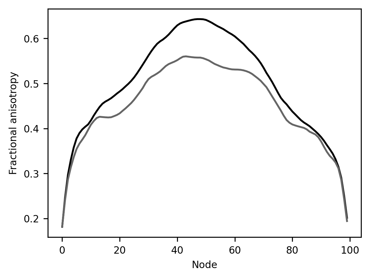
This result is rather striking! In this part of the brain, there is a substantial difference between younger children and all of the other subjects. This is a part of the white matter where there is a significant amount of development after age 10.

9.4.1.1. Exercises¶

How would you go about comparing the development of male and female subjects in this part of the brain? How would you compare younger children to the other subjects in other tracts?

To summarize, Pandas gives us a set of functionality to combine, query, and summarize data stored in tabular format. You’ve already seen here how you get from data stored in tables to a real scientific result. We’ll come back to using Pandas later in the book in the context of data analysis, and you will see more elaborate examples in which data can be selected using Pandas and then submitted to further analysis in other tools.

9.4.2. Pandas errors¶

Before we move on to the next topic, we would like to pause and discuss a few patterns of errors that are unique to Pandas and are common enough in the daily use of Pandas, that they are worth warning you about. One common pattern of errors comes from a confusion between Series objects and DataFrame objects. These are very similar, but they are not the same thing! For example, the Series objects have a very useful value_counts method that creates a table with the number of observations in the Series for every unique value. However, calling this method on a DataFrame would raise a Python AttributeError, because it doesn’t exist in the DataFrame, only in the Series. Another common error comes from the fact that many of the operations that you can do on DataFrames create a new DataFrame as output, rather than changing the DataFrame in place. For example, calling the following code:

subjects.dropna()

would not change the subjects DataFrame! If you want to retain the result of this call, you will need to assign it to a new DataFrame:

subjects_without_na = subjects.dropna()

Or use the inplace keyword argument:

subjects.dropna(inplace=True)

This pattern of errors is particularly pernicious because you could continue working with the unchanged DataFrame for many more steps leading to confusing results down the line.

Finally, errors due to indexing are also common. This is because, as you saw above, there are different ways to perform the same indexing operation, and, in contrast to indexing in Numpy arrays, indexing by rows and by columns, or indexing the order of a row (i.e., with iloc) does something rather different than indexing with the row index (i.e., with loc).

9.4.3. Additional resources¶

As mentioned at the beginning of this section, Pandas is a very popular software and there are multiple examples of its use that are available online. One resource that is quite useful is a set of snippets available from Chris Albon on his website. If you’d like to learn more about “tidy data”, you can read the paper by Hadley Wickham with the same name [Wickham, 2014].

Neuroimaging and Data Science

Manipulating tabular data with Pandas

Contents