4. Computational environments and computational containers¶

One of the challenges that you will face as you start exploring data science is that doing data science often entails combining many different pieces of software that do different things. It starts with different Python libraries. One of the reasons that people use Python for data science and scientific research, is the many different libraries that have been developed for data science in Python. This is great, but it also means that you will need to install these libraries onto your computer. Fortunately, most Python software is easy to install, but things can get a bit complicated if different projects that you use require different sets of dependencies. For example, one project might require one version of a software library, while another project might require another version of the same library. In addition, when working on a project, you often want to move all of these dependencies to a different computer. For example, to share with a collaborator or a colleague, or so that you can deploy your analysis code to a cluster or a cloud computing system. Here, we will show you two different ways to manage these kinds of situations: virtual environments and containerization.

4.1. Creating virtual environments with conda¶

A virtual environment is a directory on your computer that contains all of the software dependencies that are used in one project.

There are a few different ways to set up a working Python installation that will support running scientific software. We recommend the application that we tend to use to install scientific Python libraries and to manage virtual environments, the conda package manager. To start using that on your system, head over to the conda installation webpage and follow the instructions for your platform.

If you are working on a Linux or Mac operating system, conda should become available to you through the shell that you used in the unix section. If you are working in the Windows operating system, this will also install another shell into your system (the conda shell), and you can use that shell for conda-related operations. We refer you to an online guide from codeacademy for bringing conda into the gitbash shell, if you would like to have one unified environment to work in.

After you are done installing conda, once you start a new terminal shell, your prompt will tell you that you are in conda’s ‘base’ environment:

(base) $

Similar to our recommendation never to work in git’s main branch, we also recommend never working in conda’s base environment. Instead, we recommend creating new environments – one for each one of your projects, for example – and installing the software dependencies for each project into the project environment. Similar to git, conda also has sub-commands that do various things. For example, the conda create command is used to create new environments.

$ conda create -n my_env python=3.8

This command creates a new environment called my_env (the -n flag signifies that this is the environment’s name). In this case, we have also explicitly asked that this environment be created with version 3.8 of Python. You can explicitly specify other software dependencies as well. For example:

$ conda create -n my_env python=3.8 jupyter

would create a new virtual environment that has Python 3.8 and also has the Jupyter notebook software, which we previously mentioned in Section 1. In the absence of an explicit version number for Jupyter, the most recent version would be installed into this environment. After issuing this command, conda should ask you to approve a plan for installing the software and its dependencies. If you approve it, and once that’s done, the environment is ready to use, but you will also need to activate it to step into this environment.

$ conda activate my_env

This should change your prompt to indicate that you are now working in this environment:

(my_env) $

Once the environment is activated, you can install more software into it, using conda install. For example, to install the numpy software library, which you will learn about in Section 8, you would issue:

(my_env) $ conda install numpy

You can run conda deactivate to step out of this environment or conda activate with the name of another environment to step between environments. To share the details of an environment, or to transfer the environment from one computer to another, you can ask conda to export a list of all of the software libraries that are installed into the environment, specifying their precise version information. This is done using the conda env export command. For example, the following:

(my_env) $ conda env export > environment.yml

exports the details of this environment into a file called environment.yml. This uses the YAML markup language – a text-based format – to describe all of the software dependencies that were installed into this environment. You can also use this file to install the same dependencies on another computer on which conda has been installed by issuing:

(base) $ conda create -f environment.yml

Because the environment.yml file already contains the name of the environment, you don’t have to specify the name by passing the -n flag. This means that you can replicate the environment on your machine, in terms of Python software dependencies, on another machine. The environment.yml file can be sent to collaborators, or you can share your environment.yml in the GitHub repo that you use for your project. This is already quite useful, but wouldn’t it be nice if your collaborators could get the contents of your computer: Python software dependencies, and also operating system libraries and settings, with the code and also the data, all on their computer with just one command? With containerization, you can get pretty close to that, which is why we will talk about it next.

4.2. Containerization with Docker¶

Imagine if you could give your collaborators, or anyone else interested in your work, a single command that would make it possible for them to run the code that you ran, in the same way, with the same data and with all of the software dependencies installed in the same way. Though it is useful, conda only gets you part of the way there – you can specify a recipe to install particular software dependencies and their versions, and conda does that for you. To get all the way there, we would also need to isolate the operating system, with all of the software that is installed into it, and even data that is saved into the machine. And we would package it for sharing, or rapid deployment across different machines. The technology that enables this is called “containerization”, and one of its most popular implementations is called Docker. Like the other applications that you encountered in this chapter, Docker is a command-line interface that you run in the shell.

4.2.1. Getting started with docker¶

To install Docker, we refer you to the most up-to-date instructions on the Docker website. Once installed, you can run it on the command line1. Like git and conda, Docker also operates through commands and sub-commands. For example, the docker container command deals with containers – the specific containerized machines that are currently running on your machine (we also refer to your machine in this scenario as the host on which the containers are running).

To run a container, you will first have to obtain a Docker image. Images are the specification that defines the operating system, the software dependencies, programs, and even data that are installed into a container that you run. So, you can think of the image as a computational blueprint for producing multiple containers that are all identical to each other, or the original footage of a movie, which can be copied, edited, and played on multiple different devices.

To get an image, you can issue the docker pull command:

$ docker pull hello-world
Using default tag: latest
latest: Pulling from library/hello-world
2db29710123e: Pull complete
Digest: sha256:09ca85924b43f7a86a14e1a7fb12aadd75355dea7cdc64c9c80fb2961cc53fe7
Status: Downloaded newer image for hello-world:latest
docker.io/library/hello-world:latest

This is very similar to the git pull command. Per default, Docker looks for the image in the dockerhub registry, but you can also ask it to pull from other registries (which is the name for a collection of images). Docker tells you that it is pulling the image, and which version of the image was pulled. Much like git commits in a repo, Docker images are identified through an SHA identifier. In addition, because it is very important to make sure that you know exactly which version of the image you are using, images can be labeled with a tag. The most recent version of the image that was pushed into the registry from which you are pulling always has the tag ‘latest’ (which means that this tag points to different versions of the image at different times, so you have to be careful interpreting it!). Once you have pulled it, you can run this image as a container on your machine, and you should see the below text, which tells you that this image was created mostly so that you can verify that running images as containers on your machine works as expected.

$ docker run hello-world

Hello from Docker!
This message shows that your installation appears to be working correctly.

To generate this message, Docker took the following steps:
1. The Docker client contacted the Docker daemon.
2. The Docker daemon pulled the "hello-world" image from the Docker Hub.
   (amd64)
3. The Docker daemon created a new container from that image which runs the
   executable that produces the output you are currently reading.
4. The Docker daemon streamed that output to the Docker client, which sent it
   to your terminal.

To try something more ambitious, you can run an Ubuntu container with:
$ docker run -it ubuntu bash

Share images, automate workflows, and more with a free Docker ID:
https://hub.docker.com/

For more examples and ideas, visit:
https://docs.docker.com/get-started/

Once it’s printed this message, however, this container will stop running – That is, it is not persistent – and you will be back in the shell prompt in the host machine.

Next, as suggested in the hello world message, we can try to run a container with the image of the Ubuntu operating system, a variety of Linux. The suggested command includes two command line flags. The i flag means that the Docker image will be run interactively and the t flag means that the image will be run as a terminal application. We also need to tell it exactly which variety of terminal we would like to run. The suggested command ends with a call to the bash unix command, which activates a shell called bash. This is a popular variety of the unix shell, which includes the commands that you saw before in Section 2. This means that when we run this command, the shell on our machine will drop us into a shell that is running inside the container.

$ docker run -it ubuntu
Unable to find image 'ubuntu:latest' locally
latest: Pulling from library/ubuntu
ea362f368469: Already exists
Digest: sha256:b5a61709a9a44284d88fb12e5c48db0409cfad5b69d4ff8224077c57302df9cf
Status: Downloaded newer image for ubuntu:latest
root@06d473bd6732:/#

The first few lines indicate that Docker identifies that it doesn’t have a copy of the ubuntu image available locally on the machine, so it automatically issues the docker pull command to get it. After it’s done pulling, the last line you see in the output is the prompt of the shell inside the running Docker container. You can execute various unix commands here, including those that you have seen above. For example, try running pwd, cd and ls to see where you are and what’s in there. Once you are ready to return to your machine, you can execute the exit command, which will return you to where you were in your host operating system.

This becomes more useful when you can run some specific application within the container. For example, there is a collection of images that will run the Jupyter notebook in a container. Depending on the specific image that you run, the container will also have other components installed. For example, the jupyter/scipy-notebook image includes components of the scientific Python ecosystem (you will learn more about these in Section 8). So executing the following will start the Jupyter notebook application. Because Jupyter runs as a web application of sorts, we need to set up one more thing, which is that it will need to communicate with the browser through a port – an identified operating system process that is in charge of this communication – but because the application is isolated inside the container, if we would like to access the port on which the application is running from the host machine, we would need to forward the port from the container to the host. This is done using the -p flag, as follows:

$ docker run -p 8888:8888 jupyter/scipy-notebook

where the ‘8888:8888’ input to this flag means that the port numbered 8888 in the container (to the right of the colon) is forwarded to port 8888 in the host (to the left of the colon). When you run this you will first see Docker pulling the latest version of this image and then the outputs of Jupyter running in the container. In the end, you will see a message that looks something like this:

To access the notebook, open this file in a browser:
    file:///home/jovyan/.local/share/jupyter/runtime/nbserver-7-open.html
Or copy and paste one of these URLs:
    http://dd3dc49a5f0d:8888/?token=a90483637e65d99966f61a2b6e87d447cea6504509cfbefc
 or http://127.0.0.1:8888/?token=a90483637e65d99966f61a2b6e87d447cea6504509cfbefc

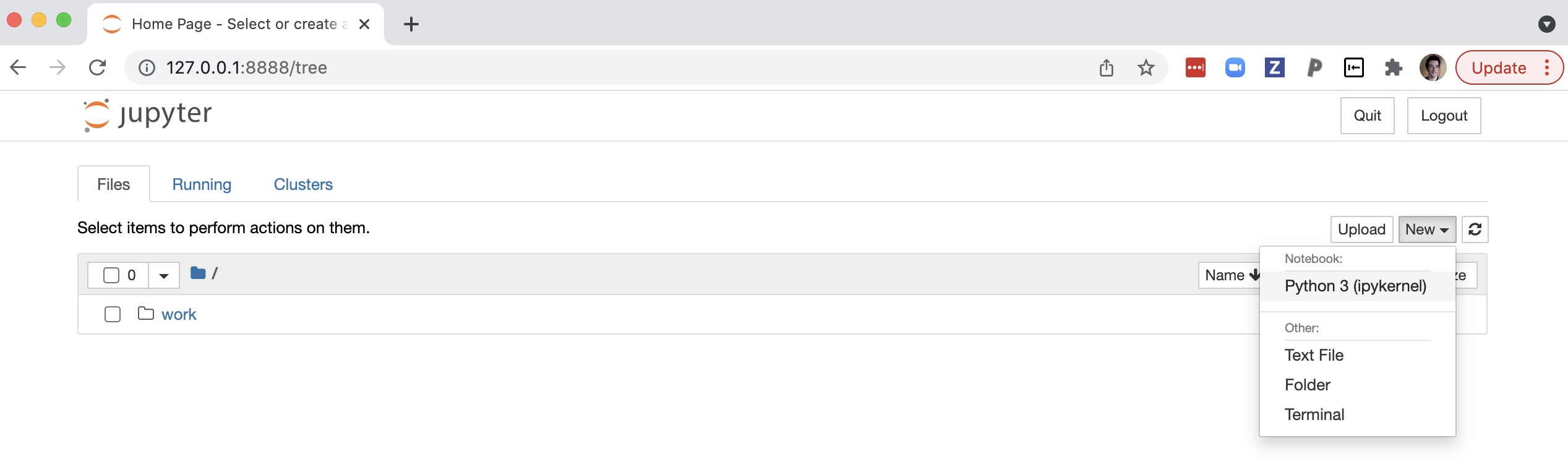
Copying the last of these URLs (the one that starts with http://127.0.0.1:8888) into your browser URL bar should open the Jupyter application in your browser and selecting the “Python 3 (ipykernel)” option would then open a Jupyter notebook in your browser, ready to import all of the components that are installed into the container.

Importantly, if you save anything in this scenario (e.g., new notebook files that you create) it will be saved into the filesystem of the container. That means that as soon as the container is stopped, these files will be deleted. To avoid this, similar to the mapping of the port in the container to a port on the host, you can also map a location in your filesystem to the container filesystem, using the -v flag. For example, the following command would mount Ariel’s projects directory (to the left of the colon) to the location /home/jovyan/work inside the container (to the right of the colon).

$ docker run -p 8888:8888 -v /Users/arokem/projects/:/home/jovyan/work jupyter/scipy-notebook

More generally, you can use the following command to mount your present working directory into that location:

$ docker run -p 8888:8888 -v $(pwd):/home/jovyan/work jupyter/scipy-notebook

If you do that, when you direct your browser to the URL provided in the output and click on the directory called work in the notebook interface, you will see the contents of the directory from which you launched Docker, and if you save new notebook files to that location, they will be saved in this location on your host, even after the container is stopped.

4.2.2. Creating a Docker container¶

One of the things that makes Docker so powerful is the fact that images can be created using a recipe that you can write down. These files are always called Dockerfile and they follow a simple syntax, that we will demonstrate next. Here is an example of a Dockerfile:

FROM jupyter/scipy-notebook:2022-01-14
RUN conda install -y nibabel

The first line in this Dockerfile tells Docker to base this image on the scipy-notebook image. The all-caps word FROM is recognized as a Docker command. In particular, on the 2022-01-14 tag of this image. This means that everything that was installed in that tag of the scipy-notebook Docker image will also be available in the image that will be created based on this Dockerfile. On the second the word RUN is also a Docker command, anything that comes after it will be run as a unix command. In this case, the command we issue instructs conda to install the nibabel Python library into the image. For now, all you need to know about nibabel is that it is a neuroimaging library that is not installed into the scipy-notebook image (and you will learn more about it in Section 12). The -y flag is here to indicate that conda will not need to ask for confirmation of the plan to install the various dependencies, which it does per default.

In the working directory in which the Dockerfile file is saved, we can issue the docker build command. For example:

$ docker build -t arokem/nibabel-notebook:0.1 .

The final argument in this command is a . that indicates to Docker that it should be looking within the present working directory for a Dockerfile that contains the recipe to build the image. In this case the -t flag is a flag for naming and tagging the image. It is very common to name images according to the construction <dockerhub username>/<image name>:<tag>. In this case, we asked docker to build an image called arokem/nibabel-notebook that is tagged with the tag 0.1, perhaps indicating that this is the first version of this image. This image can then be run in a container in much the same way that we ran the scipy-notebook image above, except that we now also indicate the version of this container.

$ docker run -p 8888:8888 -v $(pwd):/home/jovyan/work arokem/nibabel-notebook:0.1

This produces an output that looks a lot like the one we saw when we ran the scipy-notebook image, but importantly, this new container also has nibabel installed into it, so we’ve augmented the container with more software dependencies. If you would like to also add data into the image, you can amend the Dockerfile as follows.

FROM jupyter/scipy-notebook:2022-01-14
RUN conda install -y nibabel
COPY data.nii.gz data.nii.gz

The COPY command does what the name suggests, copying from a path in the host machine (the first argument) to a path inside the image. Let’s say that we build this image and tag it as 0.2:

$ docker build -t arokem/nibabel-notebook:0.2 .

We can then run this image in a container using the same command that we used above, changing only the tag:

$ docker run -p 8888:8888 -v $(pwd):/home/jovyan/work arokem/nibabel-notebook:0.2

Now, when we start the Jupyter application in our web browser, we see that the data file is already placed into the top-level directory in the container:

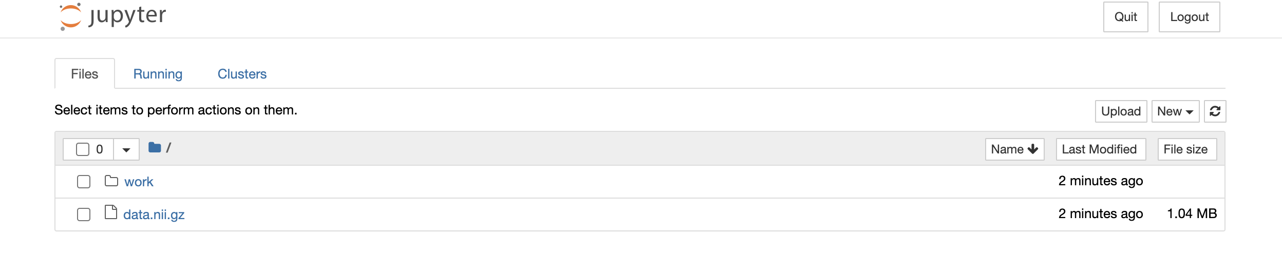
Importantly, this file is there not because the host filesystem is being mounted into the machine with the -v flag, but because we copied it into the image. This means that if we shared this image with others, they would also have that same data file in the container that they run with this image. Fortunately, Docker makes it really straightforward to share images, which we will see next.

4.3. Setting up¶

Now, that you have learned a bit about the data science environment, we are ready to set up your computer so that you can follow along and run the code in the chapters that follow. There are several options on how to do this and up-to-date instructions on installing all of the software should always be available on the book website

Here, we will focus on the simplest method, which uses Docker. Using what you’ve learned above, this should be straightforward:

$ docker pull ghcr.io/neuroimaging-data-science/neuroimaging-data-science:latest
$ docker run -p 8888:8888 ghcr.io/neuroimaging-data-science/neuroimaging-data-science:latest

After running this, you should see some output in your terminal, ending with a URL that starts with http://127.0.0.1:8888/?token=. Copy the entire URL, including the token value which follows, into your browser URL bar. This should bring up the Jupyter notebook interface, with a directory called “contents”, which contains the notebooks with all of the content of the book. Note that these notebooks are stored in the markdown format .md, but you should still be able to run them as intended1. You should be able to run through each of the notebooks (using shift+enter to execute each cell) as you follow along the contents of the chapters. You should also be able to make changes to the contents of the notebooks and rerun them with variations to the code, but be sure to download or copy elsewhere the changes that you make (or to use the -v flag we showed above to mount a host filesystem location and copying the saved files into this location), because these files will be deleted as soon as the container is stopped.

4.4. Additional resources¶

Other virtual environment systems for Python include venv. This is less focused on scientific computing, but is also quite popular.

If you are looking for options for distributing containers outside of DockerHub, one option is the GitHub container registry, which integrates well with software projects that are tracked on GitHub.

1(1,2): In some cases, you might also need to create an account on DockerHub at: https://hub.docker.com and log into this account through the application that was installed on your computer when you installed the docker command-line interface.

Neuroimaging and Data Science

Computational environments and computational containers

Contents

4. Computational environments and computational containers¶

4.1. Creating virtual environments with conda¶

4.2. Containerization with Docker¶

4.2.1. Getting started with docker¶

4.2.2. Creating a Docker container¶

4.3. Setting up¶

4.4. Additional resources¶

Neuroimaging and Data Science

Computational environments and computational containers

Contents

4. Computational environments and computational containers¶

4.1. Creating virtual environments with conda¶

4.2. Containerization with Docker¶

4.2.1. Getting started with docker¶

4.2.2. Creating a Docker container¶

4.2.3. Sharing docker images¶

4.3. Setting up¶

4.4. Additional resources¶