Validation
Contents
20. Validation
Now that we have a basic handle on overfitting, we can start thinking about ways to mitigate this problem. In this section, we’ll cover methods for validating our models. That is, obtaining better estimates of their true capabilities and identifying situations where they’re behaving in undesirable ways. While model validation doesn’t directly prevent overfitting, it plays an important indirect role. If we don’t have a good way to recognize overfitting when it happens, we’re not going to be in a great position to mitigate it.
20.1. Cross-validation
An important insight we introduced in the last section is that a model will usually perform better when evaluated on the same data it was trained on than when evaluated on an entirely new dataset. Since our models are of little use to us unless they can generalize to new data, we should probably care much more about how a model performs on new data than on data it’s already seen. That is, we want what’s known as an out-of-sample estimate of performance.
The most straightforward way to estimate out-of-sample performance is to ensure that we always train and evaluate our model on separate, independent datasets. The performance estimate obtained from the training dataset – the dataset used to fit the model – will typically suffer from overfitting to some degree; an estimate on the test dataset – the dataset that was set aside in advance for this purpose – will not, so long as the noise in this data is independent of that in the training dataset.
In practice, an easy way to construct training and test datasets with
independent errors is to randomly split a dataset in two. We’ll continue working
with the ABIDE2 data that we started working with previously. Now, we will make
use of Scikit-learn’s train_test_split utility, found in the model selection
module of the library to do the work for us. The way this function works is by
splitting an arbitrary number of array-like objects into training and testing
subsets. For every array we pass to train_test_split, we get back two: a
training set, and a test set. the train_size parameter controls the proportion
of all cases assigned to the training set, with the remainder assigned to the
test set. In the call below, X and y will each contain a randomly selected half
of the dataset. One part of the data gets designated as training data and the
other part gets designated as test data.
from sklearn.model_selection import train_test_split
X_train, X_test, y_train, y_test = train_test_split(features, y, train_size=0.5)
The practice of fitting our estimator to the training data, and then evaluating its performance on the test data is called cross-validation, and it is ubiquitous in machine learning. Here, we will evaluate the result with both the training and the test data. The performance difference between the two will tell us how badly we’re overfitting the training data. For example, we can use a linear regression model to predict age from all 1,440 structural MRI features in the ABIDE-II dataset. Notice that at the end are now calculating the \(R^2\) separately for the training sample and the testing sample:
from sklearn.linear_model import LinearRegression
from sklearn.metrics import r2_score

est = LinearRegression()

est.fit(X_train, y_train)

print(f"R^2 in training sample: ", est.score(X_train, y_train))
print(f"R^2 in test sample: ", est.score(X_test, y_test))
R^2 in training sample:  1.0
R^2 in test sample:  -0.9249385299935897
The difference here is remarkable. In the training sample, the fitted model explains 100% of the variance. In the test sample, it explains… well, none. The \(R^2\) value is negative -— implying that our model is predictively worthless! If you’re used to computing \(R^2\) by taking the square of a correlation coefficient, you might think an \(R^2\) value below 0 must be an error, but it isn’t. The standard definition of \(R^2\) as the coefficient of determination is 1 minus the ratio of the model squared errors (MSE) to the variance of the data. This allows arbitrarily large negative values because the MSE can be larger than the variance if the model is sufficiently poorly fit. Intuitively, we can have an estimator that’s so bad, we would have been better off just using the mean of the new data as our prediction, in which case the MSE would be identical to the variance, based on the definition of the variance, and \(R^2=0\).
20.1.1. When less is more
The reason our linear regression model overfits the data is that, just as in our earlier simulated example, the model has too much flexibility: the number of features is large relative to the number of available training samples. Some neuroimaging researchers might find this statement a bit surprising, seeing as the training dataset still contains over 500 subjects, and that’s a pretty large sample by the standards of most MRI experiments. But the absolute number of subjects has little bearing on the propensity of a model to overfit; what matters most is the ratio between the model’s effective degrees of freedom and the number of samples. In our case, even if we think 500 subjects is a lot (as we well might, if we’re used to working with small MRI samples), we still have far more features (1,440).
If our model is overfitting because it has too many features and not enough training data, a simple way to mitigate overfitting should be to use fewer features. Let’s see what happens if we randomly sample just 200 of the 1440 features. That way we’ll have more samples than features.
X = features.sample(200, axis='columns', random_state=99)
X_train, X_test, y_train, y_test = train_test_split(X, y, train_size=0.5, random_state=99)
est.fit(X_train, y_train)
print(f"R^2 in training sample: ", est.score(X_train, y_train))
print(f"R^2 in test sample: ", est.score(X_test, y_test))
R^2 in training sample:  0.7915613296581228
R^2 in test sample:  0.457679206912996
That looks much better! Notice that there’s still a big gap between in-sample (i.e., training) and out-of-sample (test) performance. But at least now we know that our model is capable of predicting age reasonably well in subjects it hasn’t seen before.
20.1.2. K-fold cross-validation
Splitting our data into training and test sets is a great way to evaluate our model’s out-of-sample performance, but it comes at a cost: it increases the model’s propensity to overfit the training data because we’ve halved our training sample. As a result, our model has less data to work with, which means it will be more likely to capitalize on chance and fit noise. So, at first glance, it looks like we’re stuck in a Catch-22: if we use all of our data to train the model, our estimate of the model’s true (i.e., out-of-sample) predictive performance is likely to be heavily biased. Conversely, if we split our data into separate training and testing subsets, we get a less biased estimate of the model’s true performance, but the cost is that our model won’t perform as well, because we’re giving it less data to learn from.
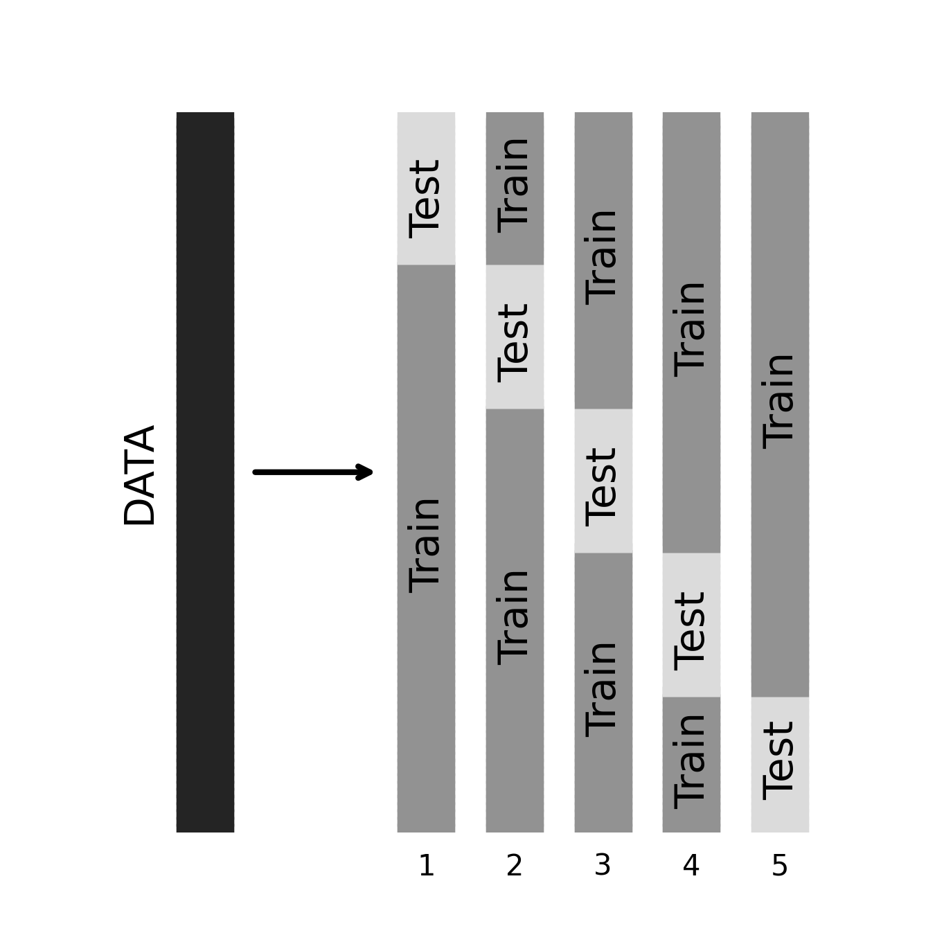
Is there a way to have our cake and eat it too? In this case, as it turns out, yes! The solution is to use a form of cross-validation known as \(k\)-fold cross-validation. The idea here is very similar to splitting our data into training and testing halves. If we set \(k\)—a parameter that represents the number of folds, or data subsets—to 2, we again end up with two discrete subsets of the data.
But now, there’s an important twist: instead of using half of the data for training and the other half for testing, we’re going to use both halves for both training and testing. The key is that we’ll take turns. First, we’ll use Half 1 to train, and Half 2 to test; then, we’ll reverse the process. Our final estimate of the model’s out-of-sample performance is obtained by averaging the performance estimates we got from the two testing halves. In this way, we’ve managed to use every single one of our data points for both training and testing, but -— critically -— never for both at the same time.
Of course, we don’t have to set \(k\) to 2; we can set it to any other value between 2 and the total sample size \(n\). At the limit, if we set \(k = n\), the approach is called leave-one-out cross-validation (because in every fold, we leave out a single data point for testing, and use the rest of the dataset for training). In practice, \(k\) is most commonly set to a value in the range of 3 - 1. There’s a long-running debate over what values of \(k\) are optimal under what conditions, and why, but we won’t get into that here. (If you ever find yourself in a situation where your results change non-trivially depending on the value of \(k\) you pick, you might want to take that as a sign that your training dataset is too small.)
20.1.3. K-folds the explicit way
To illustrate how k-folds cross-validation works, let’s implement it ourselves. First, we create \(k\) different subsets of the original dataset. Then, we loop over the \(k\) subsets and, in each case, use the current subset to test the model trained on the remaining \(k\)-1 subsets. Finally, we average over the performance estimates obtained from all \(k\) folds to obtain our overall out-of-sample performance estimate. If you’re not interested in wading through the code, you can skip to the next subsection, where we replace most of this with a single line.
First, let’s set a value for \(k\)
k = 5
We initialize placeholders for the results using numpy.zeros() and initialize
the LinearRegression object we will use for fitting.
import numpy as np
train_r2 = np.zeros(5)
test_r2 = np.zeros(5)
est = LinearRegression()
Python comes with a library for the generation of randomness (getting a computer to behave randomly is trickier than you think!). Here, we will use the shuffle function from this library, which takes a list and reorganizes it in random order. In this case, we will organize the numbers 0 thru the number of rows in X.
from random import shuffle
indices = list(range(len(X)))
shuffle(indices)
We loop over the folds. In each fold, we select every \(k\)-th index to belong to
the training set. Next, we designate all the indices not chosen to be test-set
samples as training indices (we use a list comprehension – see numref{python}
if you need a reminder). The linear regression is fit to the training data. In
each iteration, we score the model with both the training and the testing data.
When we are done, we have five estimates of \(R^2\) based on five fits of the
model.
for i in range(k):
    test = indices[i::k]
    train = [jj for jj in indices if jj not in test]
    X_train = X.iloc[train]
    X_test = X.iloc[test]
    y_train = y.iloc[train]
    y_test = y.iloc[test]

    est.fit(X_train, y_train)

    train_r2[i] = est.score(X_train, y_train)
    test_r2[i] = est.score(X_test, y_test)

print("Fold scores in training: ", train_r2)
print("Mean training R^2 over folds: ", np.mean(train_r2))

print("Fold scores in test: ", test_r2)
print("Mean training R^2 over folds: ", np.mean(test_r2))
Fold scores in training:  [0.74517282 0.75295841 0.75890923 0.75115353 0.75381255]
Mean training R^2 over folds:  0.7524013078444816
Fold scores in test:  [0.60067418 0.57296637 0.5466847  0.59152884 0.53766116]
Mean training R^2 over folds:  0.5699030510179874
Notice that the results of the 5-fold cross-validation differ from those we got when we used 50% of the data to train the model and 50% of it to test the model. Our in-sample performance is lower now (0.79 vs. 0.75), but our out-of-sample performance -— which is what we care about -— is higher (0.46 vs. 0.55).
20.1.3.1. Exercise
Why do you think out-of-sample accuracy is higher in this setting? What is the downside of having higher average out-of-sample accuracy in this case?
20.1.4. K-folds the easy way
K-folds is an extremely common validation strategy, so any machine learning
package worth its salt should provide us with some friendly tools we can use to
avoid having to reimplement the basic procedure over and over. In Scikit-learn,
the cross_validation module contains several useful utilities. We’ve already
seen train_test_split, which we could use to save us some time. But if all we
want to do is get cross-validated scores for some estimator, it’s even faster to
use the cross_val_score function. The function takes an estimator, the inputs
to the fit method, and an optional specification of the cross-validation
procedure. Integers are interpreted as the number of folds to use in a k-folds
partitioning (but there are other possible inputs to the cv key-word argument,
which we will not discuss here)
from sklearn.model_selection import cross_val_score
r2_cv = cross_val_score(est, X, y, cv=k)

print("Individual fold scores:", r2_cv)
print(f"\nMean cross-validated R^2: ", np.mean(r2_cv))
Individual fold scores: [0.60389708 0.53795077 0.56791833 0.56837218 0.55742804]

Mean cross-validated R^2:  0.567113281392003
That’s it! We were able to replace nearly all of our code above with one
function call. If you find this a little too magical, Scikit-learn also has a
bunch of other utilities that offer an intermediate level of abstraction (For
example, the sklearn.model_selection.KFold class will generate the folds for
you, but will return the training and test indices for you to loop over, rather
than automatically cross-validating your estimator).
20.1.5. Cross-validation isn’t a panacea
There’s a reason cross-validation is so popular: it provides an easy way to estimate the out-of-sample performance of just about any estimator, with minimal bias or loss of efficiency. But it isn’t magic. One problem it does nothing to solve is that of interpretation. It’s tempting to conclude from our healthy \(R^2\) above that we’ve shown that there’s some important causal relationship between brain structure and chronological age. Unfortunately, the fact that our model seems to predict age pretty well doesn’t mean we know why it’s predicting age pretty well. We don’t even know that its predictive power derives from anything to do with the brain per se. It’s possible that our brain-derived features just happen to be correlated with other non-brain features we didn’t measure, and that it’s the omitted variables that are doing the causal work for us. This might not bother us if we only cared about making good predictions. But it could be a very serious problem if we’re using machine learning as an instrument to advance scientific understanding. If it turns out that the brain features in our dataset are highly correlated with some other variable(s), that might radically change our interpretation of what our model’s doing.
As it happens, the brain variables in our dataset are correlated with at least one variable that’s very strongly associated with age: research site. The ABIDE-II dataset we’re working with contains scans from 17 sites. Let’s look at how age varies by site (we’ll use the Seaborn library for the visualization)
import seaborn as sns
import matplotlib.pyplot as plt
g = sns.catplot(x='site', y='age', data=abide_data, kind='strip', height=4, aspect=4)
g = g.set_xticklabels(rotation=30, horizontalalignment='right')
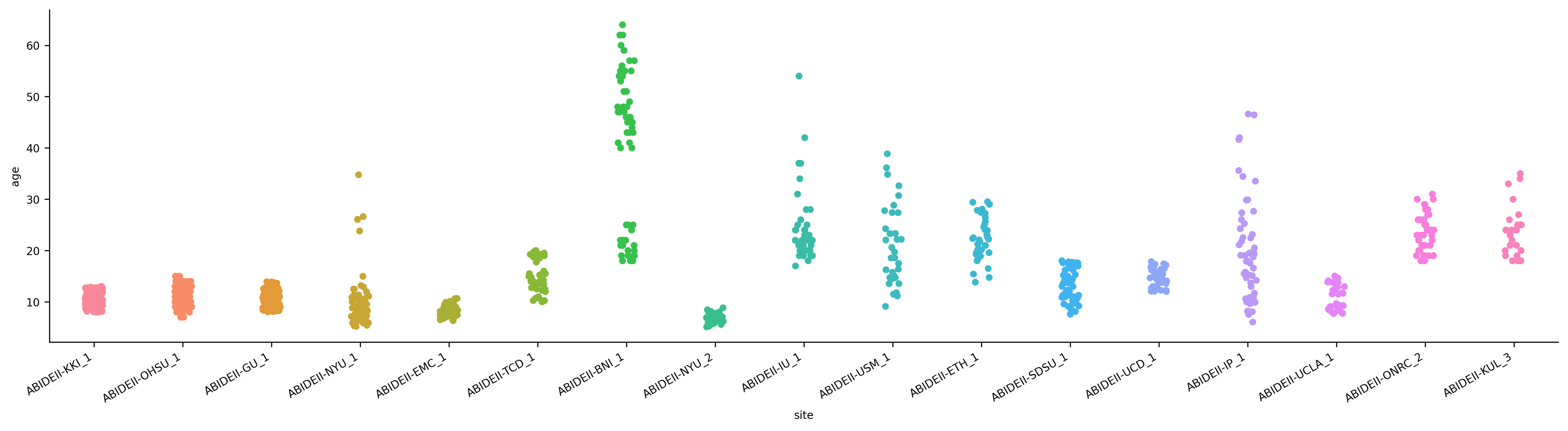
In the above plot, each strip is a different site, and each point is a single subject. As we can clearly see, sites do indeed vary wildly in their age distributions. For example, the NYU site scanned only very young children (< 10), whereas the BNI site scanned mostly adults over 40.
The fact that site differences are so big is worrisome, in one sense, as it raises the possibility that at least some of the predictive power of our model might derive from spurious associations between the research site and our brain features—i.e., that if we were to “adjust” age to account for between-site differences, the brain features might no longer do quite as much work for us in predicting age.
20.1.5.1. Exercise
There are various ways we can go about adjusting age prediction for research site. A
simple but very conservative one is to residualize age on research site. That
is, we remove all the variance in the age that can be explained by between-site
differences. To save time, we’ve included an already-residualized version of the
age variable in our dataset; it’s in the “age_resid” column. Repeat our analysis
above with 'age_resid' instead of 'age'. What does the result mean?
20.1.6. Is it all for naught?
Does this mean we’re fooling ourselves, and should just give up now? No! As noted above, this particular analysis is extremely conservative. Because the ABIDE-II sites differ so dramatically in age distributions, by controlling for research sites, we’re wiping out most of the variability in age. This would make it much harder to predict age from the brain features even if it was the site effects that were completely spurious. The root problem is that we can’t tell, just from a set of correlations, what the correct causal model is.
The reality is that causal interpretation of observational data is hard, and cross-validation doesn’t make it any easier. The question of whether or not we need to adjust for variables like site effects before examining the brain-age relationship isn’t trivial (nor is deciding how to adjust for them). For now, we’ll ignore the effects of the research site, or any other potential confounders, and just try to predict age directly from the brain variables. Just be aware that if we were planning to share these results with the rest of the world (for example, in a paper reporting what we’ve found), we’d probably need to think much more carefully about our causal assumptions, and maybe do some extra work to convince ourselves that there genuinely is a good deal of information about chronological age being carried by structural differences in people’s brains. We’ll come back to related issues toward the end of the chapter.
20.2. Learning and validation curves
So far, we’ve focused on cross-validating model performance at a single point in the dataset and parameter space. That is to say, we’re asking “how well would our fitted model do if we took it exactly as-is, changing none of its parameters, and applied it to a new dataset sampled from the same population?”
This is an important thing to know, but we can do better. If we want to get deeper insights into a model’s behavior, it’s helpful to observe the way it responds when we systematically vary the size and nature of the data, number, and type of features, model hyperparameters, etc.
In Scikit-learn, we can use the learning_curve and validation_curve
utilities to flexibly and compactly wrap most of the cross-validation
functionality we’ve already encountered. The idea behind the learning curve
is to graphically display a model’s predictive performance as a function of the
model’s experience. That is, to visualize how well it learns as the available
data grows. The validation_curve is directly analogous, except instead of
varying the size of the data, we systematically vary one of the estimator’s
parameters.
Let’s look at learning_curve in more detail. Here’s an example:
from sklearn.model_selection import learning_curve
We’ll use 100 random features as predictors.
X_subset = X.sample(100, axis=1, random_state=100)
We’ll assign a few different sizes of the samples we want to plot model
performance for and use a LinearRegressor. Note that we can’t go above 800,
because we only have ~1,000 cases, and we’re using 80% of the sample for
training.
train_sizes = [100, 200, 400, 800]
est = LinearRegression()
Next, we obtain the learning curve. as with the cross_val_score utility, the
cross-validated application of our estimator is done implicitly for us.
results = learning_curve(est, X_subset, y, train_sizes=train_sizes,
                         cv=5, shuffle=True)
sizes, train_scores, test_scores = results
The train_scores and test_scores arrays contain the performance scores for
training and testing data, respectively. The rows reflect training sizes (i.e.,
in our case, the first row gives performance \(n=100\), the second for \(n=200\), etc.)
and the columns contain the scores from the \(k\) folds of the k-folds
cross-validation procedure.
test_scores.round(2)
array([[-3.720e+01, -1.564e+02, -2.460e+00, -1.244e+01, -3.841e+01],
       [ 2.400e-01,  2.200e-01,  1.000e-01,  3.000e-01,  2.700e-01],
       [ 4.900e-01,  4.400e-01,  5.500e-01,  5.300e-01,  4.700e-01],
       [ 6.000e-01,  5.700e-01,  5.800e-01,  5.500e-01,  5.800e-01]])
This information is fairly hard to appreciate in tabular form, so let’s average performance over the columns (i.e., the \(k\) folds) and plot it as a function of the sample size.
train_mean = train_scores.mean(1)
test_mean = test_scores.mean(1)

fig, ax = plt.subplots()
ax.plot(sizes, train_mean, 'o-', label='Training')
ax.plot(sizes, test_mean, 'o-', label='Test');
ax.grid(True, axis='y')
ax.legend(fontsize=14)
ax.set_ylim(0, 1)
ax.set_xlabel('Sample size (n)')
ax.set_ylabel('$R^2$');
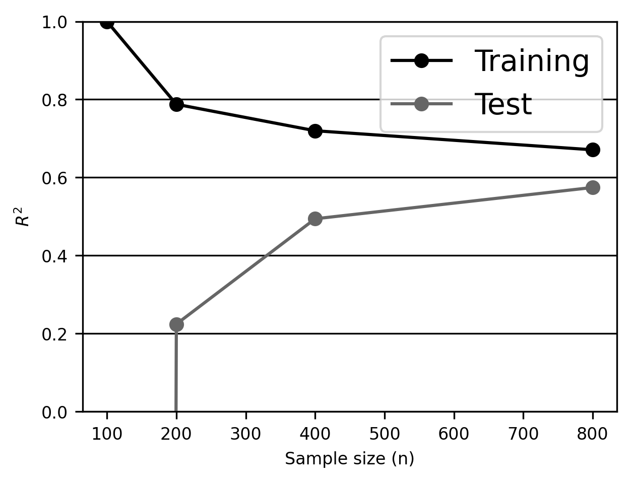
We learn several things from this plot. First, our linear regression estimator overfits with small samples: \(R^2\) in the training samples is near 1 in the training sample, but is essentially 0 in the test sample. Second, \(R^2\) in the test sample improves monotonically as the training dataset gets larger. This is a general rule: on average, a model’s out-of-sample performance should only get better as it’s trained on more data. Third, note that the training and test curves never converge, even with the largest sample we have available. This suggests that we’re still overfitting, and we might want to consider either acquiring more data (if possible) or reducing the model’s flexibility (e.g., by using fewer features, or, as we’ll see in later sections, by using a different model less prone to overfitting).
20.2.1. Training vs. test vs. validation: a note on nomenclature
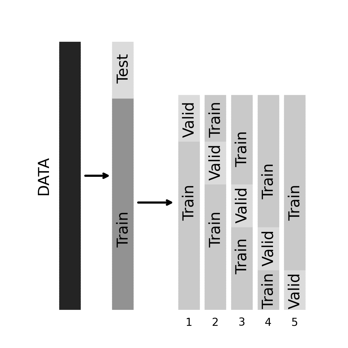
Before moving on, a quick note on nomenclature: you will sometimes hear people talk about “validation” sets rather than (or in addition to) training and test sets. What this means depends on the context. In many cases, the terms test set and validation set are used interchangeably to refer to a new dataset independently of the one the model is trained on. But sometimes, the distinction between validation and test is important. In particular, it’s common to set aside a “true” hold-out dataset in advance of any validation efforts. In such cases, the test dataset is the one we use to obtain our final estimate of performance. The validation dataset, by contrast, is technically part of the training data (in that we allow ourselves to use it to train the final model), but it’s being used for validation. When we perform a cross-validation procedure on a training set, we call the hold-out folds the validation sets.
This kind of 3-way split of our data is an excellent way to operate, as it ensures that we’re able to detect overfitting that occurs not only during model estimation but also in the model selection process. For example, if we “cross-validate” 100 models and then choose the one with the best cross-validated performance, we’re still going to overfit to some degree, and performance in the test dataset will reveal this. Next, let’s consider how we can go one further step towards systematically and automatically choosing the right model for our data.
20.2.1.1. Exercise
We’ve looked at the relationship between training dataset size and model performance. Here, you will add another dimension to the picture, and try to get a qualitative sense of how our training and validation curves vary as a function of model complexity -— in this case, we’ll operationalize this as the number of predictors our linear regression estimator gets to use.
Use the ABIDEII data to predict age given three different sizes of feature sets: 5 features, 30 features, and 100 features, which you select at random. Once again, evaluate performance for sample sizes ranging from 100 to 800.
Does our ability to predict age vary depending on how many features we use? Do the characteristics of overfitting change with the sample size?
We’ll return to a discussion of model complexity in the final section of this chapter (Section 22) when we consider the complexity of deep learning models with many thousands of parameters that can be adjusted.
20.2.2. Additional resources
Cross-validation is a very powerful tool, but it does not address all of the challenges of understanding your data. For example, as demonstrated in a paper by Gaël Varoquaux [Varoquaux, 2017], even when you do use cross-validation, the errors in your estimate of accuracy can be rather large, particularly if the sample size is not large enough. The paper is worth reading and pondering when designing studies that use machine learning methods and considering the sample size one might need.